

An RF engineer roadmap works best as a sequence of small exercises: convert power units, size a wavelength, compute a reflection, design a match, then build up to noise and a full link budget. This page sets out eight RF engineering tutorials in that order, each with a problem, a checked answer and something to try by hand, in software or on the bench.
The reading curriculum, with stages, required maths and suggested kit, is on the learn RF design page. This page is the workbook that goes with it. Do the sums by hand first, then look at the answer, and move on only when the number agrees.
The RF Engineer Roadmap as Eight Tutorials
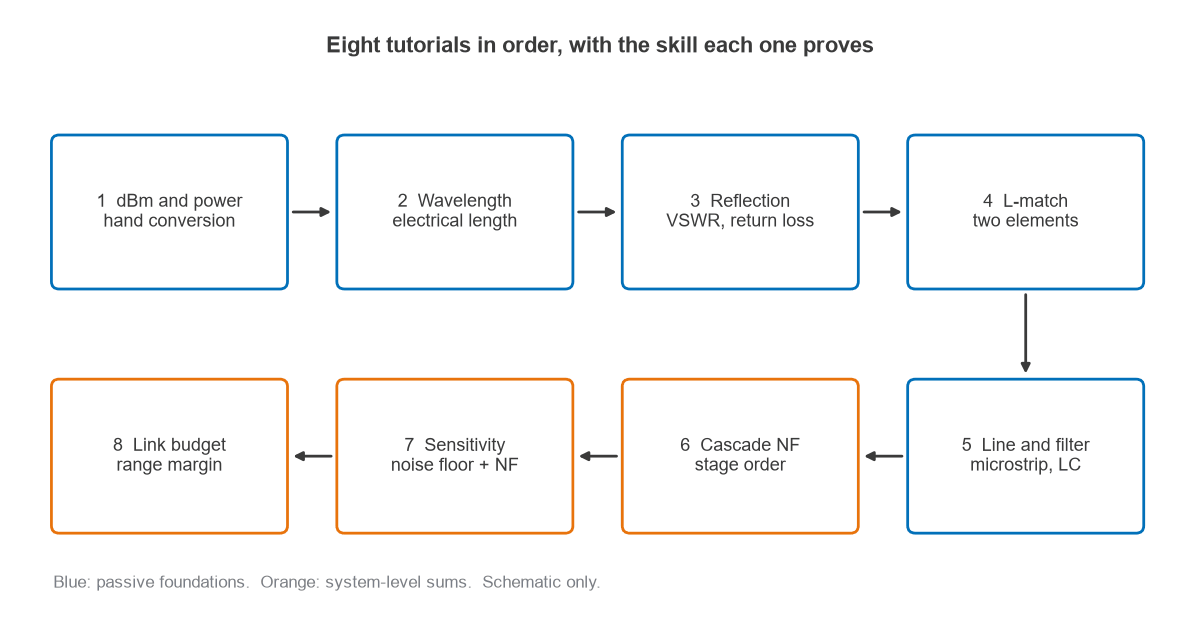
Each tutorial proves one skill that the next one needs. Tutorials 1 to 5 are passive: units, waves, reflections and matching. Tutorials 6 to 8 are system sums, where gain, noise and path loss meet. Together they cover most of what RF engineering basics means in practice, and a beginner can usually work through one a week.
| Tutorial | Skill | Read first | Tool |
|---|---|---|---|
| 1 | dBm, watts and volts | dB and dBm | Calculator |
| 2 | Wavelength, electrical length | Frequency and wavelength | Calculator |
| 3 | Reflection, VSWR, return loss | VSWR and return loss | Python or VNA |
| 4 | Two-element match | L-network matching | Matching calculator |
| 5 | Microstrip line and LC filter | LC filter design | Microstrip calculator |
| 6 | Cascaded noise figure | Cascaded noise figure | Spreadsheet |
| 7 | Noise floor and sensitivity | Thermal noise | Spreadsheet |
| 8 | Link budget | RF link budget | Spreadsheet |
Tutorial 1: Power in dBm
Power in dBm is PdBm = 10 log10(P / 1 mW). Voltage across a resistance follows from Vrms = √(PR).
Exercise. Convert 250 mW, 2 W and 1 nW to dBm. Convert 27 dBm to milliwatts. Find the RMS voltage of 2 W in 50 Ω.
Answer. 250 mW is 23.98 dBm, 2 W is 33.01 dBm and 1 nW is −60 dBm. 27 dBm is 501 mW. Two watts in 50 Ω is exactly 10 V RMS.
Hands-on. Learn the shortcuts: 3 dB doubles power, 10 dB multiplies it by ten. Try to reach 27 dBm in your head as 30 − 3, which gives 500 mW.
Tutorial 2: Wavelength and Electrical Length
Free-space wavelength is λ = c/f. A signal on a board travels more slowly, by a factor of √εeff, so electrical length is θ = 360° × ℓ√εeff / λ.
Exercise. At 433.92 MHz, find the wavelength and the length of a quarter-wave whip. Then find the electrical length of a 50 mm trace in air and on FR-4 with an effective permittivity of 3.3.
Answer. λ = 0.691 m, so a quarter wave is 172.7 mm before any end correction. The 50 mm trace is 26.1° in air and 47.3° on FR-4. That is past the λ/10 limit of 36°, so on the board it needs to be treated as a transmission line.
Hands-on. Cut a whip to length, fit it over a ground plane and, if you have a VNA, trim it while watching the reflection. The resonant length will come out a little shorter than the calculated one.
Tutorial 3: Reflection, VSWR and Return Loss
The reflection coefficient is Γ = (ZL − Z0) / (ZL + Z0). VSWR, return loss and mismatch loss all follow from its magnitude.
Exercise. For a load of 25 − j15 Ω on a 50 Ω line, find |Γ| and its angle, then VSWR, return loss and mismatch loss.
Answer. |Γ| = 0.381 at −137.7°. VSWR is 2.23, return loss is 8.38 dB and mismatch loss is 0.68 dB.
Hands-on. Repeat the sum in a few lines of Python with scikit-rf, then plot the point on a Smith chart. If you have access to a VNA, calibrate it and measure a 50 Ω load and an open.
Tutorial 4: Design an L-Match
An L-network matches a low resistance RL to a higher one RS with a series element on the low side and a shunt element on the high side. The network Q is √(RS/RL − 1). The series reactance is QRL and the shunt reactance is RS/Q.
Exercise. Match the load from Tutorial 3 to 50 Ω at 433.92 MHz using a series inductor and a shunt capacitor. Then pick the nearest standard values and find the resulting S11.
Answer. Q = 1. The series element needs +j25 Ω for the transformation and +j15 Ω more to cancel the load reactance, so the total is +j40 Ω, or 14.67 nH. The shunt capacitor has a reactance of 50 Ω, or 7.34 pF. With 15 nH and 7.5 pF, S11 at 433.92 MHz is −33.4 dB.
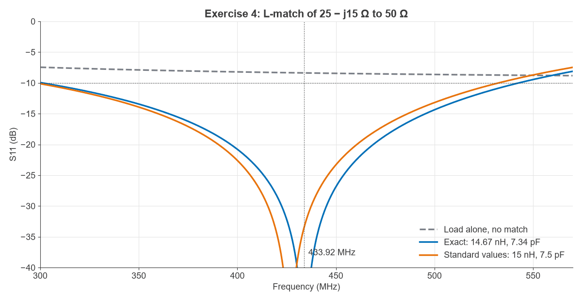
Hands-on. Check the values with the impedance matching calculator, then simulate them in one of the free RF design tools. Sweep each part by ±5% and note which one moves the dip further.
Tutorial 5: A Microstrip Line and an LC Filter
This tutorial turns numbers into copper. The Wheeler and Hammerstad synthesis equations give the width of a line, and normalised filter tables give component values.
Exercise. Find the width of a 50 Ω microstrip line on 1.6 mm FR-4 with εr = 4.3. Then design a 3-pole Butterworth low-pass filter in 50 Ω with a 500 MHz cutoff, using the C-L-C form.
Answer. The line is about 3.11 mm wide, with an effective permittivity of about 3.27 and a delay of about 6.03 ps/mm. For the filter, the prototype values are 1, 2 and 1, which give 6.37 pF, 31.8 nH and 6.37 pF.
Hands-on. Compare the width with the microstrip calculator. Lay the filter out following the RF PCB layout notes, simulate it, and if you build it, measure the cutoff. Expect part parasitics to pull it lower. The reasons are on the component parasitics page.
Tutorial 6: Cascaded Noise Figure
The Friis formula, in linear terms, is F = F1 + (F2 − 1)/G1 + (F3 − 1)/(G1G2).
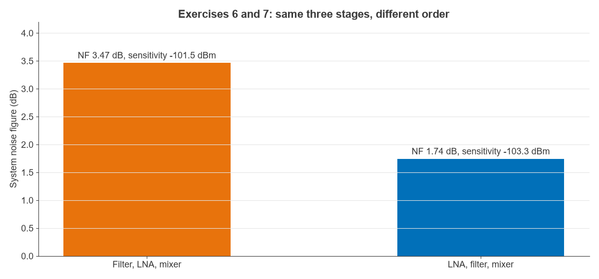
Exercise. A receiver has a filter (2 dB loss, 2 dB noise figure), an LNA (18 dB gain, 1 dB noise figure) and a mixer (7 dB loss, 10 dB noise figure). Find the system noise figure with the filter first, then with the LNA first.
Answer. Filter first gives 3.47 dB and LNA first gives 1.74 dB. Total gain is 9 dB either way.
The lower figure has a cost. An LNA placed ahead of the filter sees every strong out-of-band signal, so the order is a trade between noise and compression, not a free gain.
Hands-on. Put the Friis sum in a spreadsheet, then add 1 dB of filter loss in each order and see how much of it reaches the system noise figure.
Tutorial 7: Noise Floor and Sensitivity
Noise floor at room temperature is −174 dBm/Hz + 10 log10(B). Sensitivity adds the noise figure and the SNR the demodulator needs.
Exercise. For both receiver orders in Tutorial 6, find the sensitivity in a 1 MHz bandwidth with a required SNR of 9 dB.
Answer. The noise floor is −114 dBm. Sensitivity is −101.5 dBm with the filter first and −103.3 dBm with the LNA first.
Hands-on. Read noise figure, then take the sensitivity and bandwidth from a real receiver datasheet and work out the noise figure plus SNR they imply. With a real receiver, a lab signal generator, calibrated attenuation and a shielded enclosure, you can test such a figure as described in measuring radio performance.
Tutorial 8: A Complete Link Budget
The last tutorial uses everything so far. Received power is transmit power plus antenna gains minus path loss, and free-space path loss is 20 log10(4πd/λ).
Exercise. A 2.45 GHz link transmits 10 dBm over 100 m with a 2 dBi antenna at each end. Find the free-space path loss, the received power and the margin against the −103.3 dBm receiver above.
Answer. Path loss is 80.23 dB, received power is −66.23 dBm and margin is about 37 dB. A margin that large is needed in practice, because walls, fading and body loss take a large share of it. The antennas and propagation part of the radio architectures series covers those losses.
Hands-on. Write the budget as a spreadsheet for a radio you own, then measure received signal strength at several distances and compare.
Where the Roadmap Goes Next
After Tutorial 8, pick one circuit block and design it fully. The RF amplifiers section is a good choice, and the RF circuit design basics article walks through a first LNA stage with real values. Readers who want more theory behind each tutorial can use the RF engineering fundamentals article and the RF fundamentals hub. For the job itself, see what an RF engineer does.
Frequently Asked Questions
What is the roadmap to become an RF engineer?
Learn units and wavelengths first, then transmission lines and matching, then S-parameters, noise and linearity, and finally circuit blocks and radio systems. An engineering degree is the usual entry route to the job, and practical work on real boards is what makes the theory stick.
How long do these RF engineering tutorials take?
At one tutorial a week, the eight take about two months alongside other study. Tutorials 4 and 5 usually take longest, particularly if you build the hardware.
Do I need lab equipment for these tutorials?
No. Every exercise can be done with a calculator and free software. A low-cost VNA adds a lot from Tutorial 3 onwards, because a measured result that disagrees with the sum teaches more than one that agrees.
Are there free online RF engineering courses?
Many universities publish lecture material, and the pages linked here are free. See the RF design guide for the full topic list and RF design books for longer reading.
Related Topics
Continue with the learn RF design curriculum, the RF calculators and the RF design guide. For interview practice on the same material, try the RF interview questions.