LC Filter Design: Butterworth, Chebyshev and Elliptic

Lumped LC filter design is the method of building a filter from discrete inductors and capacitors by scaling a normalized low-pass prototype, a ladder of tabulated g-values, to the required cutoff frequency and system impedance. To design an LC low-pass filter, choose the response type and order from the stopband requirement, look up or calculate the g-values, then convert each one to a capacitance or inductance with two simple scaling formulas.

The method works from a few hundred kilohertz up to roughly 1 to 2 GHz, where component parasitics start to dominate and distributed structures such as the ones in microstrip filter design take over. This page sits under the RF filters hub and assumes the specification terms (cutoff, ripple, stopband attenuation) covered in RF filter specifications.

Butterworth, Chebyshev and Elliptic Responses

The three classical responses trade passband flatness against how fast the attenuation rises above cutoff.

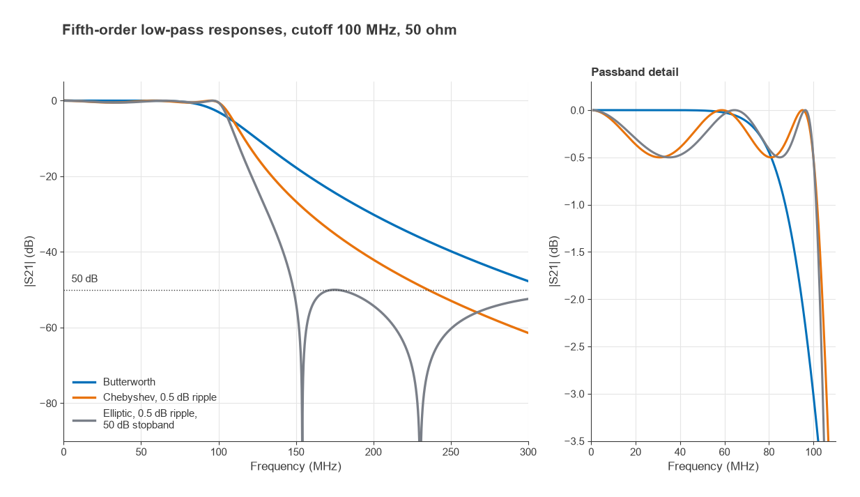
S21 of fifth-order Butterworth, 0.5 dB Chebyshev and elliptic low-pass filters with 100 MHz cutoff, plus passband detail — Figure 1: Fifth-order low-pass responses with a 100 MHz cutoff in 50 ohm. At 200 MHz the Butterworth gives 30.1 dB and the Chebyshev 42.0 dB; the elliptic design reaches 50 dB near 149 MHz.

Butterworth is maximally flat. The insertion loss is |S₂₁|⁻² = 1 + (f/f_c)²ⁿ, so the response has no ripple and is exactly 3.01 dB down at f_c. Attenuation far above cutoff rises at 20n dB per decade.
Chebyshev allows a fixed passband ripple L_r in exchange for a steeper skirt. Here f_c is the ripple bandwidth: the response is L_r dB down at cutoff, not 3 dB. Group delay varies more across the passband than for a Butterworth filter of the same order.
Elliptic (Cauer) filters add transmission zeros in the stopband, made from series or shunt resonators inside the ladder. They give the sharpest transition for a given order, but the stopband attenuation bounces back up between zeros instead of rising monotonically.

For a fifth-order design with a 100 MHz cutoff, the Butterworth filter gives 30.1 dB of attenuation at 200 MHz and the 0.5 dB Chebyshev gives 42.0 dB. An elliptic design with 0.5 dB ripple and a 50 dB minimum stopband reaches 50 dB at about 149 MHz. The Chebyshev needs about 235 MHz to reach the same level and the Butterworth about 316 MHz.

Choosing the order

The minimum order for an attenuation of A dB at a stopband frequency f_s follows directly from the response equations:

Butterworth: n ≥ log₁₀(10^A/10 − 1) / [2 log₁₀(f_s/f_c)]
Chebyshev: n ≥ cosh⁻¹√[(10^A/10 − 1)/(10^L_r/10 − 1)] / cosh⁻¹(f_s/f_c)

Asking for 40 dB at twice the cutoff frequency gives n ≥ 6.64 for Butterworth, so a seventh-order filter, and n ≥ 4.82 for a 0.5 dB Chebyshev, so a fifth-order filter. Two fewer reactive parts is a real saving in loss, board area and tuning effort.

Prototype g-Values

A low-pass prototype is a ladder normalized to a 1 Ω source and a cutoff of 1 rad/s. Each element value g_k is either a shunt capacitance in farads or a series inductance in henries. The ladder can start with a shunt capacitor (the pi form) or with a series inductor (the T form); both give the same response.

Butterworth values have a closed form:

g_k = 2 sin[(2k − 1)π / 2n], k = 1 … n, with g₀ = g_n+1 = 1

Chebyshev values are computed recursively. With β = ln[coth(L_r/17.37)], γ = sinh(β/2n), a_k = sin[(2k − 1)π/2n] and b_k = γ² + sin²(kπ/n):

g₁ = 2a₁/γ, g_k = 4a_k−1a_k / (b_k−1g_k−1)

For odd n the load is 1 Ω, matching the source. Even-order Chebyshev prototypes need a load other than 1 Ω, which is one reason odd orders are used far more often in 50 Ω systems. Elliptic g-values have no simple closed form and are normally taken from published tables or filter synthesis software.

Element	Butterworth, n = 5	Chebyshev 0.5 dB, n = 5
g₁	0.618	1.706
g₂	1.618	1.230
g₃	2.000	2.541
g₄	1.618	1.230
g₅	0.618	1.706
g₆ (load)	1.000	1.000

Impedance and Frequency Scaling

Two substitutions turn the prototype into real components for a system impedance R₀ and cutoff frequency f_c, with ω_c = 2πf_c:

Shunt capacitor: C_k = g_k / (ω_cR₀)
Series inductor: L_k = g_kR₀ / ω_c

The same prototype also gives high-pass and band-pass filters through frequency transformations. For a high-pass filter, each series inductor becomes a series capacitor of 1/(ω_cg_kR₀) and each shunt capacitor becomes a shunt inductor of R₀/(ω_cg_k). For a band-pass filter centred on ω₀ with fractional bandwidth FBW, each series inductor becomes a series LC resonator with L = g_kR₀/(ω₀FBW) and C = FBW/(ω₀g_kR₀), and each shunt capacitor becomes a parallel resonator with C = g_k/(ω₀FBW R₀) and L = FBW R₀/(ω₀g_k).

Worked Example: Fifth-Order 100 MHz Low-Pass Filter

The steps below design a fifth-order Butterworth low-pass filter for a 50 Ω system with a 3 dB cutoff of 100 MHz, in the shunt-capacitor-first form.

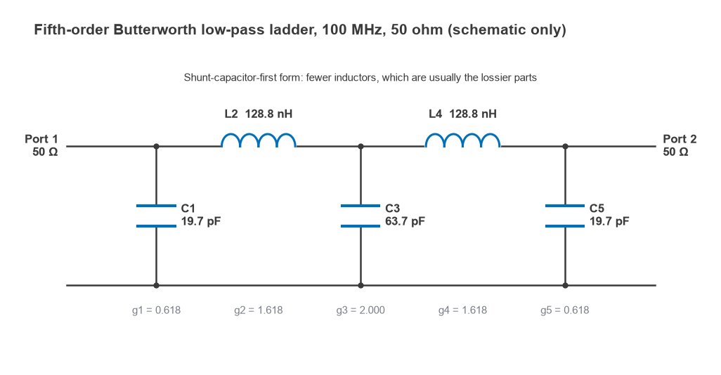
Ladder schematic of a fifth-order Butterworth low-pass filter with 19.7 pF, 128.8 nH and 63.7 pF elements — Figure 2: The worked fifth-order Butterworth ladder in shunt-capacitor-first form, with the g-value behind each element (schematic only).

Compute ω_cR₀ = 2π × 10⁸ × 50 = 3.1416 × 10¹⁰, and R₀/ω_c = 50 / 6.2832 × 10⁸ = 7.958 × 10⁻⁸.
C₁ = C₅ = 0.618 / 3.1416 × 10¹⁰ = 19.67 pF.
L₂ = L₄ = 1.618 × 7.958 × 10⁻⁸ = 128.8 nH.
C₃ = 2.000 / 3.1416 × 10¹⁰ = 63.66 pF.
Round to available values: 20 pF, 130 nH and 62 pF from the E24 series.
Simulate the rounded design with realistic component Q, then build and measure it.

The pi form uses three capacitors and two inductors. Since inductors are usually the lossier and more variable parts, starting with a shunt capacitor is the common choice. Rounding to E24 values moves the 3 dB point to about 101.0 MHz and changes the loss at 100 MHz from 3.01 dB to 2.79 dB. At 200 MHz the rounded filter still gives 30.2 dB of rejection, so the change is small.

The same steps applied to the 0.5 dB Chebyshev g-values give C₁ = C₅ = 54.30 pF, L₂ = L₄ = 97.85 nH and C₃ = 80.88 pF. The Chebyshev version uses larger capacitors and smaller inductors, and its response is 0.5 dB down at 100 MHz rather than 3 dB.

Component Q and Parasitic Effects

Real inductors and capacitors have loss, described by their unloaded quality factor Q_u = X/R_s. A series inductor with Q_L has a series resistance ωL/Q_L, and a shunt capacitor with Q_C has a parallel conductance ωC/Q_C. Small chip inductors around 100 MHz often have Q values somewhere between 30 and 80, while good RF capacitors are typically in the hundreds, so inductor loss usually dominates. Check the Q factor curves in each part’s datasheet at the frequency of interest.

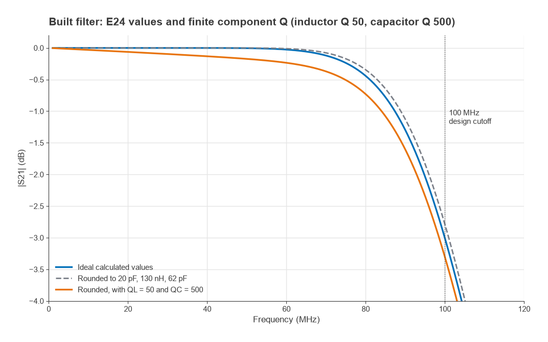
Passband S21 of the 100 MHz filter with ideal values, E24 rounded values, and with inductor Q 50 and capacitor Q 500 — Figure 3: Rounding to E24 values moves the 3 dB point to about 101 MHz. Adding inductor Q of 50 and capacitor Q of 500 (constant with frequency) raises the loss at 80 MHz from 0.35 dB to 0.73 dB.

With an inductor Q of 50 and a capacitor Q of 500 (held constant with frequency for simplicity), the rounded 100 MHz filter shows 0.03 dB of loss at 10 MHz, 0.17 dB at 50 MHz and 0.73 dB at 80 MHz, against 0.35 dB at 80 MHz for the lossless version. The loss grows toward cutoff because the stored energy, and so the current in the lossy elements, rises there. Loss in the stopband changes very little: 30.3 dB at 200 MHz instead of 30.2 dB.

Band-pass filters are far more sensitive to Q

For a band-pass filter, Cohn’s approximation gives the midband loss as

IL ≈ 4.343 Σg_k / (FBW · Q_u) dB

A third-order 0.5 dB Chebyshev band-pass filter (g = 1.596, 1.097, 1.596) with 5% fractional bandwidth and resonators of Q_u = 100 has an estimated loss of 4.343 × 4.289 / (0.05 × 100) = 3.73 dB. Halving the bandwidth doubles the loss. This is why narrow band-pass filters move to cavities, ceramic resonators, or SAW and BAW filters, whose resonator Q is far higher than a chip inductor’s.

Self-resonance and layout parasitics

Every inductor has a self-resonant frequency (SRF) set by its winding capacitance, and every capacitor has one set by its lead and pad inductance. Above the SRF the part behaves as the opposite element, which can open up a spurious passband well above cutoff. A practical rule is to pick inductors with an SRF several times the highest stopband frequency that matters. Pad capacitance, via inductance in the shunt capacitor returns and coupling between adjacent inductors all shift the response; the effects are covered in RF component parasitics and RF PCB layout. Mounting inductors at right angles to each other reduces mutual coupling.

From Calculation to Hardware

Hand calculation gets the topology and starting values. Before ordering boards, simulate the ladder with vendor component models or measured S-parameters for each part, then include the pad and via parasitics. On the bench, a vector network analyzer shows S₂₁ and S₁₁ directly. A cutoff that comes out low usually points to extra shunt capacitance from pads; poor stopband depth often points to a shared ground via or coupling between inductors. The impedance matching view of the filter is also useful: |S₁₁| in the passband shows how far the built filter departs from the design.

Frequently asked questions

How do you design an LC low-pass filter?

Choose a response type and calculate the order needed to meet the stopband attenuation. Take the prototype g-values for that order, then scale them with C = g/(2πf_cR₀) and L = gR₀/(2πf_c). Round to standard values, simulate with realistic component Q and parasitics, and confirm on a network analyzer.

Butterworth vs Chebyshev: which should I use?

Use Butterworth when flat amplitude and well-behaved group delay matter more than selectivity, for example ahead of a data converter carrying wideband modulation. Use Chebyshev when the stopband requirement is tight and a small passband ripple is acceptable; it often saves one or two elements for the same rejection.

When is an elliptic filter worth the extra parts?

When an interferer or harmonic sits close to the passband edge and must be rejected by a fixed amount. The transmission zeros can be placed on or near the unwanted frequency. The cost is resonators inside the ladder, which are more sensitive to component tolerance, and a stopband that rises and falls rather than increasing steadily.

Up to what frequency do lumped LC filters work?

Chip-component LC filters are common up to roughly 1 to 3 GHz, depending on part size and the order required. Above that, element values become small enough that pad and via parasitics are comparable to the intended values, and distributed microstrip or stripline filters are usually easier to control.