

Part 12, Zero-IF Receivers, DC Offset and I/Q Imbalance, showed how removing the IF simplifies a receiver while creating new problems near DC. Direct RF sampling goes one step further. The mixer and LO disappear from the signal path, and an ADC digitizes the RF signal itself, either in its first Nyquist zone or in a higher zone by deliberate undersampling. Everything that used to be analog (frequency translation, channel filtering, even some of the band selection) becomes arithmetic.
This is the architecture most people mean when they talk about software-defined radio in its full sense. It builds directly on Part 5, ADCs and Receivers, and it borrows the jitter analysis from Part 11. What changes is scale: converters sampling at several gigasamples per second, input frequencies in the gigahertz range, and digital processing that has to keep up with all of it.
Nyquist Zones and Undersampling
A converter sampling at fs cannot tell the difference between an input at f and inputs at |f − kfs| for any integer k. The frequency axis divides into Nyquist zones, each fs/2 wide. Zone 1 runs from 0 to fs/2, zone 2 from fs/2 to fs, zone 3 from fs to 3fs/2, and so on. Every zone folds onto zone 1. Signals in even-numbered zones arrive spectrally inverted; signals in odd zones keep their orientation.
Undersampling uses this deliberately. A bandpass signal confined to one zone can be sampled at a rate far below twice its carrier frequency, as long as the sample rate exceeds twice the signal’s bandwidth and the band does not straddle a zone edge. The penalty is that an anti-alias filter must now be a bandpass filter that removes everything in all the other zones, because each of them folds onto the same output frequencies. The ADC’s analog input bandwidth must also extend to the zone in use, and its distortion and jitter performance at that frequency, not at the sample rate, is what counts.
Worked example: where do the signal and its harmonics land?
An ADC samples at fs = 3 GSPS and the wanted signal is centred at 2.6 GHz. Zone 2 runs from 1.5 to 3.0 GHz, so the signal is in zone 2.
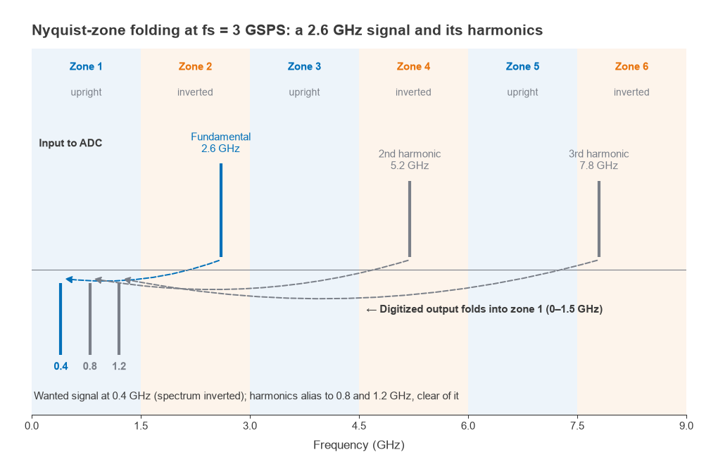
- Fundamental: 3.0 − 2.6 = 0.4 GHz, spectrally inverted.
- Second harmonic at 5.2 GHz: subtract fs to get 2.2 GHz, which lies in zone 2, so the alias is 3.0 − 2.2 = 0.8 GHz.
- Third harmonic at 7.8 GHz: subtract 2fs to get 1.8 GHz, alias 3.0 − 1.8 = 1.2 GHz.
The harmonics alias to 800 MHz and 1.2 GHz, well clear of the wanted signal at 400 MHz. A frequency plan always checks this, along with the folded positions of interleaving spurs at fs/2 − fin and fs/4 ± fin for interleaved converters, and any clock-related spurs. Moving the sample rate by a few percent is often the cheapest way to move a harmonic out of the band.
Noise, Processing Gain and Equivalent Noise Figure
An RF ADC’s SNR is specified over the full Nyquist band, fs/2. When the wanted channel is much narrower, the digital filters that follow discard most of that noise. The improvement is the processing gain:
PG = 10log((fs/2) / Bch)
The same idea is captured by noise spectral density, NSD = −SNR − 10log(fs/2) dBFS/Hz, and by an equivalent noise figure for the converter, which lets the ADC be placed in a Friis cascade like any other stage:
NFADC = PFS − SNR − 10log(fs/2) + 174 dB
where PFS is the full-scale input power in dBm and 174 comes from kT at 290 K, −174 dBm/Hz.
Worked example: from ADC datasheet to system noise figure
Take an ADC at 3 GSPS with a measured SNR of 58 dBFS at the input frequency and a full-scale input of +1 dBm.
- Nyquist bandwidth: 1.5 GHz, so 10log(1.5 × 10⁹) = 91.76 dB.
- NSD = −58 − 91.76 = −149.76 dBFS/Hz, or +1 − 149.76 = −148.76 dBm/Hz.
- NFADC = −148.76 + 174 = 25.24 dB.
- For a 20 MHz channel, PG = 10log(1.5 × 10⁹ / 20 × 106) = 10log(75) = 18.75 dB, so the in-channel SNR at full scale is 58 + 18.75 = 76.75 dB.
A 25 dB noise figure is far too high for a receiver on its own, so an LNA goes in front. With an LNA of 1.5 dB noise figure and 25 dB gain, the Friis equation gives
F = F1 + (F2 − 1)/G1 = 1.413 + (334.2 − 1)/316.2 = 1.413 + 1.054 = 2.466
which is 3.92 dB. The converter still contributes more than the LNA. Adding more gain lowers the cascade noise figure but reduces the largest signal the system can accept before the ADC clips: every dB of gain ahead of the converter costs a dB of input-referred full scale. That trade between sensitivity and blocking is the central design decision in a direct-sampling receiver, and it is usually settled by the strongest out-of-channel signal that the bandpass filter lets through.
Clock Jitter at Gigahertz Inputs
The jitter-limited SNR from Part 11, SNR = −20log(2πfintj), depends on the input frequency, not on the sample rate. That is bad news for undersampling. At fin = 2.6 GHz with tj = 50 fs rms, 2π × 2.6 × 109 × 50 × 10−15 = 8.17 × 10⁻⁴, so the jitter limit is 61.8 dB. That is only a few dB better than the 58 dB converter in the example above, and it means the clock contributes a meaningful share of total noise. At 100 fs the limit falls to 55.7 dB and the clock dominates.
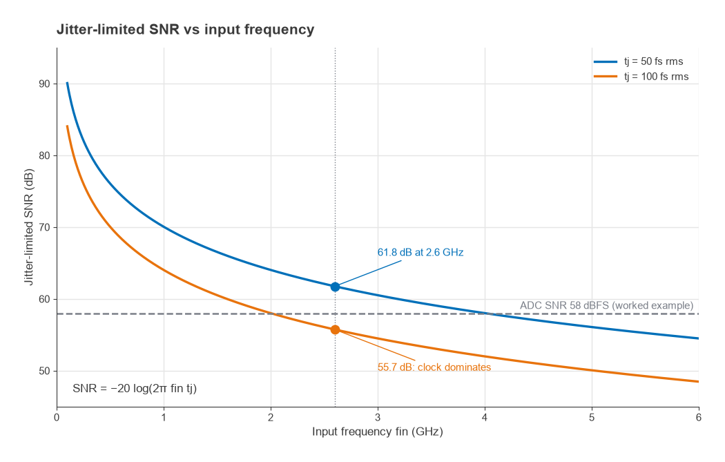
The relevant jitter is the total of the ADC’s internal aperture jitter and the external clock jitter, combined as the root sum of squares. Clock jitter integrated over a wide offset range matters, because the converter samples every edge, but the far-out phase noise floor often contributes most of it. This is why direct-sampling systems use clock sources with very low wideband noise, often a low-noise VCO or crystal-referenced PLL followed by careful filtering, and why clock distribution is laid out with the same care as the RF input.
Close-in phase noise on the sample clock also behaves like LO phase noise in a superhet: it is transferred onto every sampled signal, so a strong blocker acquires a phase noise skirt that can cover a weak adjacent channel. Reciprocal mixing, discussed in Part 10, does not go away just because the LO has been replaced by a sample clock.
Digital Downconversion
The ADC delivers a wideband real data stream at gigasamples per second. A digital downconverter (DDC) turns it into something a baseband processor can use:
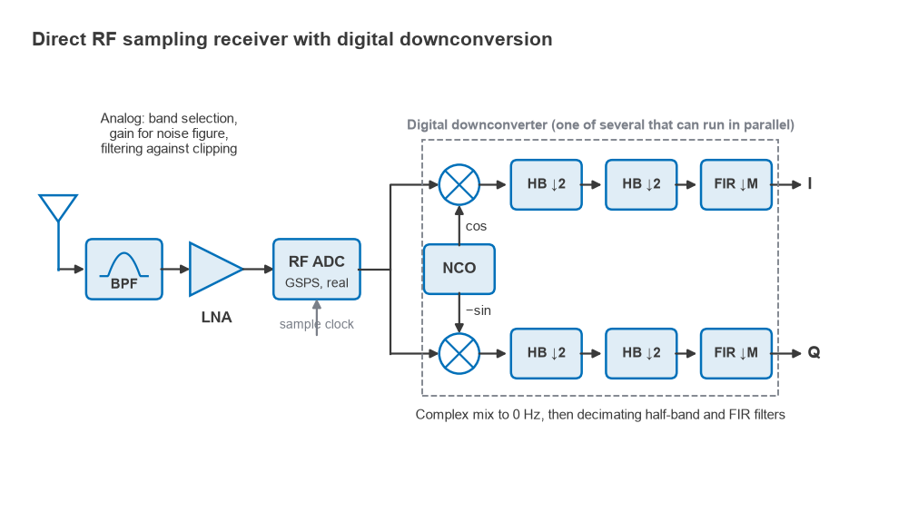
- A numerically controlled oscillator generates digital sine and cosine at the wanted channel’s aliased frequency.
- A complex multiplier mixes the data to zero frequency, producing I and Q.
- A chain of decimating filters, often half-band stages and a final FIR, removes everything outside the channel and lowers the sample rate.
Because the mixing is digital, the I and Q paths have identical gain and an exact 90° relationship. The DC offset, flicker noise and I/Q imbalance problems of Part 12 do not arise in the DDC. NCO spurs replace them, set by phase accumulator truncation and the size of the sine lookup, but these are deterministic and can be pushed below the converter’s own spurs by using enough bits. Several DDCs can run in parallel on the same ADC output, each tuned to a different channel or band, which is how one converter serves multiple carriers.
What Software-Defined Radio Actually Buys
The term software-defined radio is used loosely. At one end it describes any radio with a configurable digital baseband. At the other it describes a receiver in which the only hardware between antenna and processor is a filter, an amplifier and a converter. Direct RF sampling moves a design towards that second end.
| Aspect | Superhet or zero-IF | Direct RF sampling |
|---|---|---|
| Frequency translation | Analog mixers and LO | Sampling and NCO |
| Channel selection | IF or baseband analog filters | Digital decimation filters |
| Reconfiguration | Limited by analog filter bandwidths | Limited by ADC bandwidth and processing |
| Main limit on dynamic range | Mixer linearity and IF filtering | ADC SNR, SFDR and clock jitter |
| Power consumption | Lower for narrow channels | Higher; ADC and digital filters run at GSPS rates |
Flexibility is the real gain. A single hardware design can cover several bands, change channel bandwidths and support new waveforms through firmware. The costs are power, since converters and logic running at gigahertz rates consume watts rather than milliwatts, and dynamic range, because a wideband ADC sees every signal in its band at once and its full scale is shared among all of them. Strong blockers anywhere in the passband reduce the headroom left for weak signals. The analog front end therefore still matters. It just has fewer jobs: band selection, enough gain to set the noise figure, and enough filtering to keep the converter out of clipping. Those jobs belong to the front-end module.
Next in the Series
Part 14, Front-End Modules, Duplexers and Switches, looks at that hardware between the antenna and the converter: how PAs, LNAs, filters and switches are combined into modules, what duplexer isolation has to achieve in an FDD radio, and how switch insertion loss and linearity enter the system budget.