

An impedance matching calculator is a design tool that finds the inductor and capacitor values which transform a load impedance into the conjugate of the source impedance at one frequency. Enter the frequency, the source impedance ZS and the load impedance ZL, and the calculator below returns every valid two-element L-network, the nearest standard E12 or E24 component values, and low-pass Pi and T networks for a loaded Q that you choose, with the result drawn on a Smith chart.
The equations behind it are the standard closed-form L-section results found in microwave textbooks, extended to complex sources. They assume ideal, lossless lumped components, so the output is a starting point for a schematic or simulation rather than a finished bill of materials. The theory is covered in more depth in impedance matching in RF design, L-network matching and Pi and T matching networks.
How to Use the Calculator
Enter impedances as resistance and reactance in ohms. A capacitive load has a negative reactance, so a 12.5 Ω resistor in series with 3.32 pF at 2.4 GHz is entered as RL = 12.5 and XL = −20. If the source is a 50 Ω system, leave XS at zero. The network is described from the load side: “element at load” is the component connected directly to the load, and “element at source” is the one connected to the source. Series elements are in line with the signal, shunt elements go to ground.
The return loss column is computed with the rounded E-series values in place of the exact ones, so it shows directly how much match is lost by buying standard parts. The Q field only affects the Pi and T results. The Smith chart is normalized to the reference impedance you enter (50 Ω by default) and shows each L-network path from the load to the conjugate of the source impedance.
L-network solutions
| # | Element at load | Element at source | Nearest standard values | Return loss with standard values |
|---|
Low-pass Pi and T networks
| Network | Source side | Middle | Load side |
|---|
Which L-Network Topologies Can Match a Load
An L-network has one series element and one shunt element, and there are two ways to arrange them: shunt element at the load with the series element toward the source, or series element at the load with the shunt element toward the source. Each arrangement has two solutions, one with a positive and one with a negative intermediate reactance, so there are at most four L-networks for any pair of impedances.
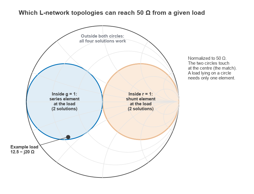
For a real source resistance RS, the Smith chart shows which arrangements work. If the normalized load lies inside the r = 1 circle (RL > RS), only the shunt-at-load form can reach the centre. If it lies inside the g = 1 circle (load conductance GL > 1/RS), only the series-at-load form works. Outside both circles all four solutions exist. A load that already sits on one of the circles needs a single element.
L-Network Equations Used by the Calculator
The calculator matches ZL = RL + jXL to the conjugate of ZS = RS + jXS, which is the condition for maximum power transfer. Write the load admittance as YL = 1/ZL = GL + jBL and the source admittance as YS = GS + jBS.
Shunt element at the load
The shunt susceptance must bring the real part of the load impedance up to RS. Requiring Re{1/(GL + jBt)} = RS gives the total susceptance
Bt = ±√(GL/RS − GL2), so the added shunt element is B = Bt − BL.
The series element then cancels what remains: X = −Im{1/(GL + jBt)} − XS.
A real solution requires GL ≤ 1/RS, which is the “outside the g = 1 circle” condition when the source is real.
Series element at the load
Here the series reactance moves the load onto the circle where the conductance equals GS. Requiring Re{1/(RL + jXt)} = GS gives
Xt = ±√(RL/GS − RL2), so the added series element is X = Xt − XL.
The shunt element then cancels the remaining susceptance: B = −Im{1/(RL + jXt)} − BS.
This form requires RL ≤ 1/GS. With a real 50 Ω source that simply means RL ≤ 50 Ω. Subtracting XS and BS is what lets the same equations handle a complex source such as a transistor output.
From reactance to component values
With ω = 2πf, a positive series reactance is an inductor L = X/ω and a negative one is a capacitor C = −1/(ωX). A positive shunt susceptance is a capacitor C = B/ω and a negative one is an inductor L = −1/(ωB). The calculator then picks the nearest E12 or E24 value on a logarithmic scale, so 2.297 pF becomes 2.2 pF and 1.914 nH becomes 2.0 nH. Real inductors and capacitors are sold in finer steps at low values, so the E-series result is a conservative check, not a rule.
Pi and T Networks With a Chosen Q
An L-network has no free parameter: its loaded Q is fixed at Q = √(Rhigh/Rlow − 1). A third element adds one degree of freedom, which can be used to raise Q and narrow the bandwidth, for example to add harmonic rejection at a power amplifier output. The calculator treats a Pi as two back-to-back L-networks meeting at a virtual resistance
Rv = max(RpS, RpL)/(Q2 + 1), with Q1 = √(RpS/Rv − 1) and Q2 = √(RpL/Rv − 1)
where RpS = 1/GS and RpL = 1/GL are the parallel-equivalent resistances. The shunt susceptances are Q1/RpS and Q2/RpL, and the series reactance is (Q1 + Q2)Rv. The T network is the dual: Rv = min(RS, RL)(Q2 + 1), series reactances Q1RS and Q2RL, and a shunt susceptance (Q1 + Q2)/Rv. Both are given in low-pass form. Any reactive part of the terminations is absorbed by subtracting BS and BL from the Pi end capacitors, or XS and XL from the T end inductors. If Q is below √(Rmax/Rmin − 1) no virtual resistance exists, and the calculator says so.
Worked Example: 12.5 − j20 Ω to 50 Ω at 2.4 GHz
Take a load of ZL = 12.5 − j20 Ω, equivalent to 12.5 Ω in series with 3.32 pF at 2.4 GHz, and a 50 Ω source. These are the calculator’s default inputs.
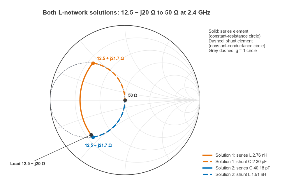
- Load admittance: YL = 0.02247 + j0.03596 S, so RpL = 44.5 Ω. Because GL = 0.02247 S is greater than 1/50 = 0.02 S, the load is inside the g = 1 circle and only the series-at-load form works.
- Intermediate reactance: Xt = ±√(12.5 × 50 − 12.52) = ±√468.75 = ±21.65 Ω.
- Solution 1: X = 21.65 − (−20) = +41.65 Ω, a series inductor of 41.65/(2π × 2.4 GHz) = 2.76 nH. The impedance becomes 12.5 + j21.65 Ω, whose admittance is 0.0200 − j0.03464 S. The shunt element is B = +0.03464 S, a capacitor of 2.30 pF.
- Solution 2: X = −21.65 + 20 = −1.65 Ω, a series capacitor of 40.2 pF, which moves the load to 12.5 − j21.65 Ω. The shunt element is B = −0.03464 S, an inductor of 1.91 nH.
| Network | Exact values | E24 values | Return loss at 2.4 GHz with E24 values | Band with return loss > 10 dB (exact values) |
|---|---|---|---|---|
| L solution 1 | series 2.76 nH, shunt 2.30 pF | 2.7 nH, 2.2 pF | 24.1 dB | 2.12 to 2.66 GHz |
| L solution 2 | series 40.2 pF, shunt 1.91 nH | 39 pF, 2.0 nH | 28.8 dB | 2.00 to 3.22 GHz |
| Pi, Q = 3 | 3.98 pF, 1.93 nH, 1.80 pF | 3.9 pF, 2.0 nH, 1.8 pF | 21.4 dB | 2.25 to 2.54 GHz |
| T, Q = 3 | 4.06 nH, 2.24 pF, 3.81 nH | not computed | not computed | 2.22 to 2.55 GHz |
For the Pi, Rv = 50/(32 + 1) = 5 Ω, Q1 = 3 and Q2 = √(44.5/5 − 1) = 2.81. The load-side capacitor needs a total of 2.81/44.5 = 0.0632 S, but the load already supplies 0.0360 S, so only 0.0272 S (1.80 pF) is added. For the T, Rv = 12.5 × 10 = 125 Ω, Q1 = 1.22 and Q2 = 3. The load-side inductor reactance is 3 × 12.5 + 20 = 57.5 Ω because it must also cancel the load’s −20 Ω. The bandwidth columns model the load as a fixed 12.5 Ω resistor in series with 3.32 pF, so the load’s own reactance also changes with frequency.
Bandwidth and the Effect of Standard Values
All of the networks match perfectly at 2.4 GHz with exact values, but they differ away from it. The two L solutions have the same loaded Q at the design frequency, yet in this example solution 2 holds 10 dB return loss over about 1.2 GHz while solution 1 covers about 0.54 GHz. The difference comes from how each element’s reactance changes with frequency relative to the load’s own capacitance. The single-frequency equations cannot predict it, so always sweep candidate networks in a simulator or with the return loss relationships. The Pi and T with Q = 3 are deliberately narrower, at about 0.3 GHz.
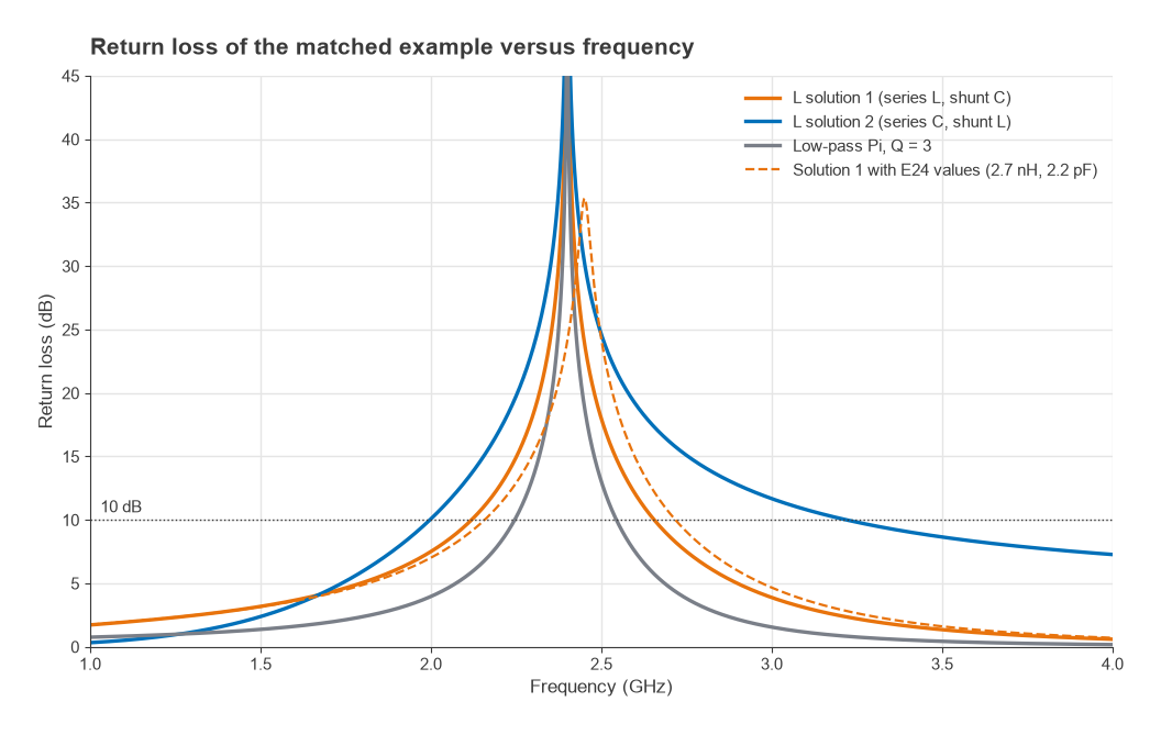
Rounding to E24 values moves the centre of solution 1 up to about 2.45 GHz and leaves 24.1 dB of return loss at 2.4 GHz, a reflected power of about 0.4 percent. That is usually acceptable. For wider-band requirements, see broadband matching and the quarter-wave transformer; for distributed alternatives at higher frequencies, see stub matching.
Accuracy Limits
The equations are exact for ideal components at a single frequency. Real parts differ in three ways. Chip inductors and capacitors have parasitics and self-resonant frequencies, so a 40 pF capacitor at 2.4 GHz may be close to or above its self-resonance and behave quite differently from its nominal value. Components have finite Q, and the loss they add grows with the loaded Q of the network, which matters most for high transformation ratios. Pads, traces and vias add their own reactance, which at gigahertz frequencies can be comparable to a 2 nH inductor. For a production design, use the calculator to choose a topology and approximate values, then re-optimize with the vendor’s S-parameter models and the board layout included.
Frequently Asked Questions
What component values match my load?
Enter the frequency, source impedance and load impedance in the calculator. It lists every valid L-network with exact inductor and capacitor values, the nearest E12 or E24 values and the return loss those standard parts give. For a 12.5 − j20 Ω load at 2.4 GHz and a 50 Ω source, one answer is a 2.76 nH series inductor followed by a 2.30 pF shunt capacitor.
Why are there two L-network solutions?
The matching condition fixes the magnitude of the intermediate reactance or susceptance but not its sign, so there is one solution on each side of the real axis of the Smith chart. One is usually low-pass in character and the other high-pass. Choose between them on DC path, harmonic rejection, bandwidth and component availability.
Can the calculator match a complex source?
Yes. It matches the load to the conjugate of the source impedance by subtracting the source reactance or susceptance from the element next to the source. This is the case for an amplifier output or input whose optimum impedance is not 50 Ω.
Why does my matched network measure differently on the board?
The calculator assumes ideal parts with no pads or traces. Component parasitics, self-resonance, finite Q and layout reactance all shift the result, and the effect grows with frequency. Measure the actual load on a VNA at the reference plane where the network will sit, then tune.
Related Topics
This calculator belongs to the impedance matching section of the RF design guide. The design theory is covered in L-network matching and Pi and T matching networks. Antenna matching shows the same networks applied in products, reflection coefficient explains the return loss figures, and more tools are collected on the RF calculators page.