

A SAR sensor in mobile phones is a capacitive proximity sensor that tells the modem when a body is close to a transmitting antenna, so the phone can lower its transmit power and stay within specific absorption rate (SAR) limits. It does not measure SAR. It detects nearby material from a small change in capacitance, often using the antenna itself as the sensing electrode, and its job is regulatory compliance.
What Is a SAR Sensor in Mobile Phones?
SAR stands for specific absorption rate: the RF power absorbed per unit mass of tissue, in watts per kilogram (W/kg). At a point in tissue:
SAR = σE2 / ρ
Here σ is tissue conductivity in S/m, E is the RMS electric field in V/m and ρ is density in kg/m3.
Why a Phone Measures Proximity Rather Than SAR
SAR cannot be measured inside a phone. A laboratory finds it by scanning a field probe through tissue-simulating liquid in a phantom. A phone in service has no such probe and no knowledge of the tissue around it.
So the problem is solved in advance. Certification measures SAR for each band, position and power level, and those results fix a table of allowed power levels. Conducted power is already known from the power detector and modem settings, so proximity is the one missing input.
Capacitive Proximity Sensing With the Antenna as Electrode
A capacitive sensor measures the capacitance from an electrode to ground, typically with a low-frequency drive in the tens to hundreds of kilohertz. Tissue is lossy and has high permittivity, so a body near the electrode adds capacitance.
The change is small. A parallel-plate estimate, C = ε0A/d, gives 0.35 pF for a 4 cm2 electrode facing a body 10 mm away, 0.71 pF at 5 mm and 0.18 pF at 20 mm. Fringing fields raise those figures, but the order of magnitude holds. Against a 30 pF baseline, 0.35 pF is only 1.2%, so sensing ICs need offset compensation and fine resolution.
Using the radiator as the electrode places the detection zone where the RF fields are strongest, with no separate pad. A dedicated flex electrode is the alternative.
RF Decoupling the Sense Line From the Antenna
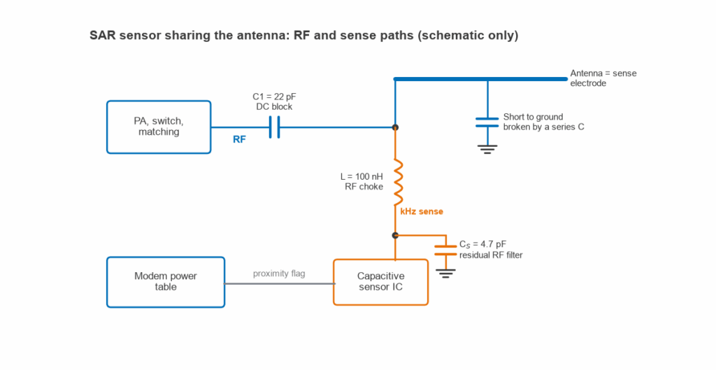
One metal structure now carries two signals several decades apart in frequency. RF must not reach the sensor, and the sensor must not see the RF path’s low-frequency connections to ground. Figure 1 shows the usual arrangement.
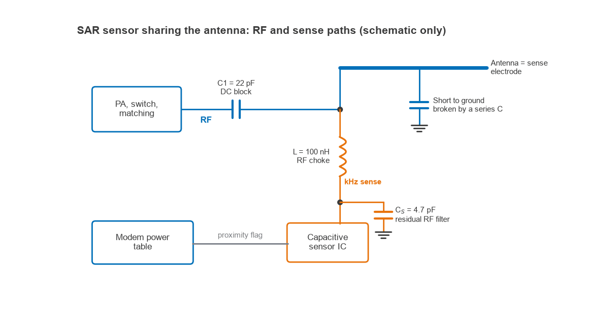
- Series inductor (RF choke). Passes the sense signal and presents a high impedance at RF.
- Series capacitors (DC blocking). Isolate the electrode from the feed and from any short to ground at low frequency, while acting as near shorts at RF.
- Shunt capacitor at the sensor pin. Filters residual RF that gets past the choke.
Worked Example: Reactance at 900 MHz and 2 GHz
Take L = 100 nH, C1 = 22 pF, CS = 4.7 pF and a 200 kHz sense frequency, using XL = 2πfL and XC = 1/(2πfC).
| Frequency | XL, 100 nH | XC, 22 pF | XC, 4.7 pF |
|---|---|---|---|
| 200 kHz | 0.13 Ω | 36.2 kΩ | 169 kΩ |
| 900 MHz | 565 Ω | 8.0 Ω | 37.6 Ω |
| 2 GHz | 1,257 Ω | 3.6 Ω | 16.9 Ω |
The inductor is negligible to the sensor and large at RF, and C1 does the reverse. As a shunt element on a 50 Ω line, with an assumed Q of 30, the choke adds 0.02 dB of loss at 900 MHz and under 0.01 dB at 2 GHz.
At 23 dBm, a 50 Ω line carries 4.47 V peak. The L and CS divider passes XC/(XL − XC): 0.32 V peak at 900 MHz (−22.9 dB) and 0.06 V peak at 2 GHz (−37.3 dB). Real inductors fall short of this near self-resonance, and antenna mismatch raises the voltage, so a detuned case should be checked.
C1 and CS add to the baseline the sensor must null out, and C1 joins the antenna matching network, so both belong in the tuning from the start. The impedance matching calculator helps with that check, and layout guidance is in PCB antenna design.
How a Phone Backs Off Transmit Power
When the sensor reports proximity, the modem applies a lower maximum power for that antenna and band. This is a cap: closed-loop power control still runs below it. The 3GPP specifications call this kind of reduction power management maximum power reduction (P-MPR). The 5G RF front end and front-end module articles show where power is set.
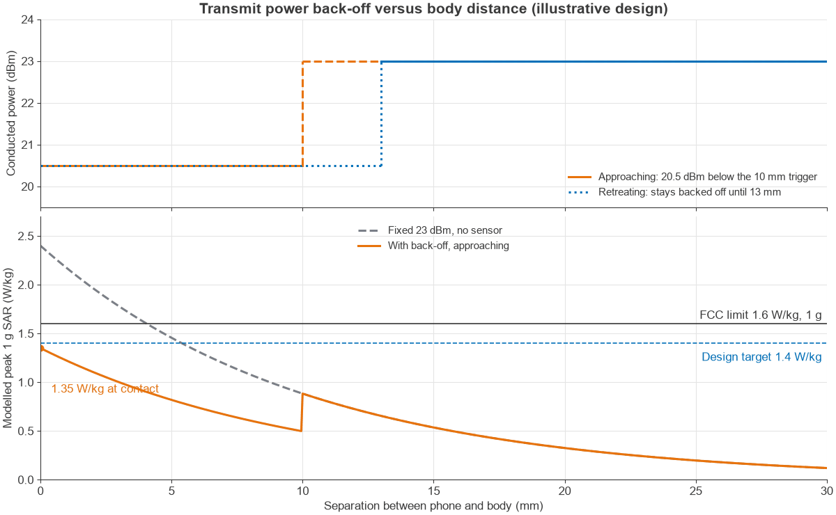
The trip point uses hysteresis, with a longer release distance than trigger distance, so a hand near the threshold does not make the power chatter.
Worked Example: Back-Off in dB, Average Power and Duty
Assume 23 dBm (200 mW) maximum conducted power, with an illustrative lab result of 2.4 W/kg over 1 g at contact, transmitting continuously. The design target is 1.4 W/kg, leaving margin under a 1.6 W/kg limit. SAR scales linearly with time-averaged power.
- Required back-off = 10 log10(2.4 / 1.4) = 2.34 dB. In 0.5 dB steps, that rounds up to 2.5 dB.
- Backed-off power = 23 − 2.5 = 20.5 dBm, or 112 mW. SAR = 2.4 × 10−0.25 = 1.35 W/kg.
- Modelled with a decay of 1/e per 10 mm, full-power SAR reaches 1.4 W/kg at 5.4 mm, so a 10 mm trigger distance is comfortable. At 10 mm, full power gives 0.88 W/kg.
- Duty: on a TDD carrier with an assumed 25% uplink duty, 23 dBm during the slots averages 50 mW (17 dBm). SAR is then 2.4 × 0.25 = 0.6 W/kg with no back-off.
- Allowed average power for the target = 200 × 1.4 / 2.4 = 117 mW (20.7 dBm). At full power, that equals a maximum duty of 58%.
A phone that can only transmit part of the time starts with an inherent reduction in average power, so the sensor may be needed only for high uplink duty or for several simultaneous transmitters.
SAR Limits: 1.6 W/kg Over 1 g and 2.0 W/kg Over 10 g
The two numbers quoted most often use different averaging masses, so they are not interchangeable.
| Framework | Local limit, general public | Averaging mass | Limbs |
|---|---|---|---|
| US FCC, 47 CFR 1.1310 | 1.6 W/kg | Any 1 g cube | 4 W/kg over 10 g (extremities, pinnae) |
| ICNIRP 2020 | 2 W/kg (head and torso) | 10 g cube | 4 W/kg over 10 g |
| EU, Recommendation 1999/519/EC | 2 W/kg (head and trunk) | Any 10 g | 4 W/kg over 10 g |
The FCC and ICNIRP also set a 0.08 W/kg whole-body limit for the general public. The FCC allows averaging over up to 30 minutes for general population limits, and ICNIRP averages local SAR over 6 minutes. A 1 g cube has a side of about 1 cm and a 10 g cube about 2.15 cm, and at the limit they absorb 1.6 mW and 20 mW respectively. Values from the two frameworks cannot be compared directly.
The EU Recommendation is not itself binding on member states. Phones sold in the EU show conformity with the Radio Equipment Directive using product standards such as EN 50360 and EN 50566, with EN 62209 measurement methods. Under 47 CFR 2.1093 a phone is a portable device, with its radiating structure within 20 cm of the body. Above 6 GHz, ICNIRP uses absorbed power density in place of SAR.
These figures are stated as regulatory limits only. The sensor exists so that a design meets them in every tested position.
Effect on Uplink Throughput
Back-off costs nothing when the phone is below its power cap, as it usually is close to a base station. The effect appears at the cell edge, where the phone needs all of its power.
A Shannon estimate, C/B = log2(1 + SNR), gives the scale of a 2.5 dB reduction:
| Uplink SNR before back-off | Before (b/s/Hz) | After 2.5 dB (b/s/Hz) | Loss |
|---|---|---|---|
| 3 dB | 1.58 | 1.09 | 31% |
| 20 dB | 6.66 | 5.84 | 12% |
In practice the effect often appears as fewer resource blocks: at constant power spectral density, 2.5 dB less power supports 56% of the bandwidth. In link budget terms, with a path loss exponent of 3.5, it shortens uplink range by about 15%. See antenna parameters and power amplifier classes for the factors that set the starting point.
False Triggers and Calibration
A capacitive sensor reports capacitance, not people, and its errors carry different costs.
- False triggers. Water, metal surfaces or a case can look like a body, and the phone loses uplink margin for no reason.
- Missed detection. A slow approach, or booting against a body, can be absorbed into the baseline. This is the compliance risk, so designs bias toward back-off.
- Drift. Temperature and humidity move the baseline, and on a 1% signal small drifts matter.
- RF coupling. Residual transmit energy can shift the reading, so sampling away from bursts helps. See RF coexistence.
In the factory, offsets and thresholds are set per design and checked per unit. In the field, firmware tracks the baseline slowly, freezes tracking during proximity and can fall back to the backed-off state if the reading looks invalid.
Certification tests this behaviour. FCC test reports for tablets under KDB 616217 show labs finding the trigger distance against a phantom, then testing SAR at full power just inside it so that production units still comply.
Time-Averaged SAR as a Newer Approach
SAR limits are defined over time, so a phone can control average power instead of capping every burst. Time-averaged SAR control tracks transmitted energy over a rolling window and keeps it within a budget. A proximity input may still select the budget.
The FCC’s October 2018 TCB workshop slides listed interim maximum averaging times of 100 seconds below 3 GHz and 60 seconds for 3 to 6 GHz. They also describe measuring SAR at a not-to-exceed continuous average power and validating the algorithm with specific test sequences. These are workshop slides rather than rules, so current FCC KDB publications should be checked for any filing.
Continuing the example, 117 mW over 100 s allows 11.7 J per window. With a 50 mW reserve, a continuous uplink can hold 200 mW for 44 s of each 100 s, because 200T + 50(100 − T) = 11,667 mJ gives T = 44.4 s. Short uploads run at 23 dBm with no back-off at all.
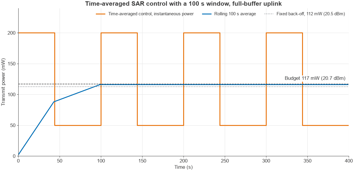
The cost is a modem algorithm that must be validated, and a long continuous upload still settles at the budgeted average.
Frequently asked questions
Is a SAR sensor the same as the proximity sensor that turns off the screen?
No. The screen-off sensor is usually an optical sensor near the earpiece. A SAR sensor is capacitive, sits at or near the antenna, and feeds the modem power control rather than the display.
What does a SAR sensor in a mobile phone actually measure?
It measures capacitance from an electrode to ground. A body nearby raises that capacitance by a fraction of a picofarad, and crossing a threshold changes the allowed transmit power. It does not measure SAR, RF field or absorbed power.
Do all phones have a SAR sensor?
No. Whether one is needed depends on maximum power, band, antenna position, duty and how a design measures against the limits. A design with enough margin in every test position can comply with fixed power settings or with time averaging alone.
Related topics
See antennas, antennas and propagation in radio design, RF design applications and the RF calculators.