Vector Network Analyzer (VNA) Basics

A vector network analyzer (VNA) is a test instrument that measures how a device reflects and transmits RF signals, recording both magnitude and phase so that the result is a full set of S-parameters rather than a power reading. A VNA measures return loss, impedance, gain or insertion loss, phase and group delay of filters, amplifiers, cables, antennas and matching networks across a swept frequency range.

Phase is what makes it “vector”. Because the VNA knows the phase of each wave, it can mathematically remove the systematic errors of its own hardware and cables during calibration, which a scalar instrument cannot. This page explains how a VNA works, which settings matter, and what limits low-cost instruments. It belongs to the RF measurement and test section.

How a VNA Works

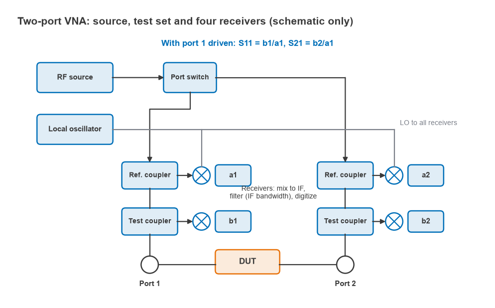
A two-port VNA contains four main blocks:

Source. A synthesized signal swept or stepped across the measurement band, with adjustable power.
Test set. A switch routes the source to port 1 or port 2, and directional couplers or bridges at each port separate the incident wave from the reflected wave.
Receivers. Each sampled wave is mixed down to a low intermediate frequency, filtered and digitized. The incident waves are labelled a₁ and a₂; the reflected or transmitted waves are b₁ and b₂.
Processor. Computes the wave ratios, applies the calibration error model and displays the results.

Many VNAs have four receivers, one for each wave. Lower-cost designs use three receivers, with a single reference receiver shared by both ports, which limits the calibration methods available.

Block diagram of a two-port VNA with source, port switch, couplers, four receivers a1 b1 a2 b2 and the DUT — Figure 1: A two-port VNA with a switched source, reference and test couplers at each port, and four receivers. With port 1 driven, S11 = b1/a1 and S21 = b2/a1 (schematic only).

Measuring S-Parameters

With port 1 driven and port 2 terminated in the analyzer’s matched load, the forward parameters are ratios of measured waves:

S₁₁ = b₁/a₁, S₂₁ = b₂/a₁

The switch then drives port 2 to give S₂₂ = b₂/a₂ and S₁₂ = b₁/a₂. Because each S-parameter is a ratio, the absolute source power cancels, and so does most of the source’s level variation with frequency. From the four complex values the analyzer derives the quantities engineers normally read:

Return loss = −20 log₁₀|S₁₁| dB, and VSWR = (1 + |S₁₁|)/(1 − |S₁₁|)
Input impedance Z_in = Z₀(1 + S₁₁)/(1 − S₁₁), usually displayed on a Smith chart
Gain or insertion loss = 20 log₁₀|S₂₁| dB
Group delay = −dφ₂₁/dω, from the slope of the S₂₁ phase

The theory behind these definitions is on the S-parameters page, and the relationship between return loss and VSWR on VSWR and return loss.

How to Use a VNA, Step by Step

Set the start and stop frequencies to cover the band of interest plus enough margin to see the behaviour either side.
Choose the number of points. Enough points are needed to resolve sharp features: a resonance with a 1 MHz bandwidth needs a step well below 1 MHz.
Set the source power. Keep it low enough that an amplifier under test stays linear and the receivers do not compress, and high enough to keep traces clean.
Set the IF bandwidth for the dynamic range needed (see below).
Attach the test cables and adapters that will be used for the measurement, then calibrate at the ends of those cables using a calibration kit. Settings changed after calibration may invalidate it.
Verify the calibration by measuring a known device, such as a through line, an open or a precision attenuator.
Connect the device under test without flexing the cables more than necessary, and read the results with markers.
Save the data as a Touchstone file for simulation, together with the instrument settings.

Calibration types (SOLT, TRL and others) and the error terms they correct are covered on VNA calibration. If the device sits on a fixture, the fixture can be removed afterwards by de-embedding.

IF Bandwidth and Dynamic Range

The IF bandwidth (IFBW) is the bandwidth of the digital filter that follows each receiver’s mixer. Noise power in the receiver is proportional to that bandwidth, so the noise floor moves by 10 log₁₀(IFBW₁/IFBW₂) dB when the IFBW changes. Reducing the IFBW by a factor of ten lowers the noise floor by 10 dB, but the receiver needs longer to settle at each point, so the sweep slows by about the same factor.

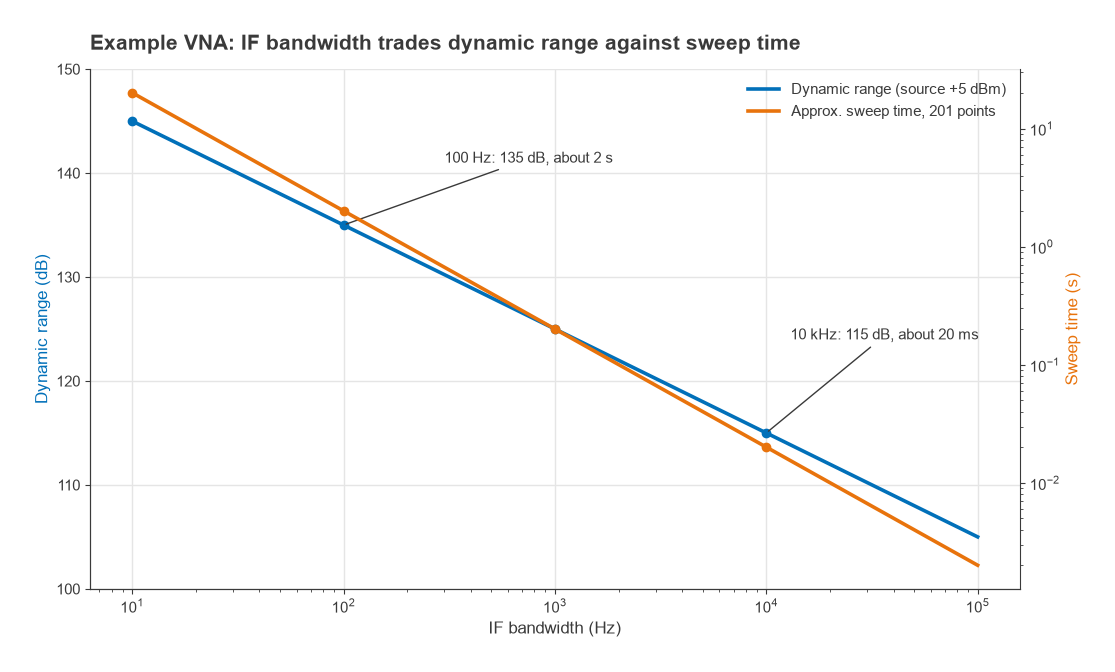
Dynamic range and sweep time versus IF bandwidth for an example VNA with a -110 dBm floor at 10 kHz — Figure 2: For an example analyzer with a -110 dBm floor at 10 kHz IFBW and +5 dBm source, each tenfold IFBW reduction adds 10 dB of dynamic range and multiplies sweep time by about ten.

Dynamic range is the difference between the maximum power the receiver handles and its noise floor, or, for a transmission measurement, between the source power and the noise floor. It sets the deepest rejection the VNA can measure.

Worked example: measuring a filter stopband

Take an example analyzer with a receiver noise floor of −110 dBm at 10 kHz IFBW and a source power of +5 dBm. The transmission dynamic range is 5 − (−110) = 115 dB.

Simulated S21 of a fifth-order 1 GHz band-pass filter measured at 10 kHz and 100 Hz IF bandwidth against its true response — Figure 3: Simulated measurement of a fifth-order 1 GHz band-pass filter. At 10 kHz IFBW the stopband disappears into noise near -115 dB; at 100 Hz the trace follows the true response to about -130 dB.

IF bandwidth	Noise floor	Dynamic range	Approx. time for 201 points
10 kHz	−110 dBm	115 dB	20 ms
1 kHz	−120 dBm	125 dB	0.2 s
100 Hz	−130 dBm	135 dB	2 s
10 Hz	−140 dBm	145 dB	20 s

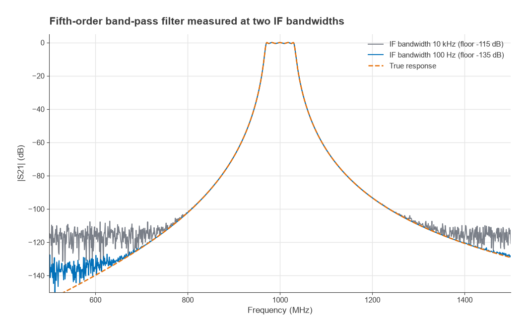
The sweep times assume roughly 1/IFBW per point and ignore fixed overheads, so real instruments are somewhat slower. A fifth-order band-pass filter centred on 1 GHz has a true rejection of about 123 dB at 700 MHz and 140 dB at 600 MHz. At 10 kHz IFBW, the measured trace flattens into noise around −115 dB and hides that stopband. At 100 Hz it follows the true response down to about −130 dB. A practical approach is to sweep fast with a wide IFBW while tuning, then narrow the IFBW, or narrow it only in the stopband segment, for the final measurement.

Averaging also lowers trace noise, but it does not lower the noise floor the way a narrower IFBW does; it smooths the noise around its mean.

Directivity and Reflection Accuracy

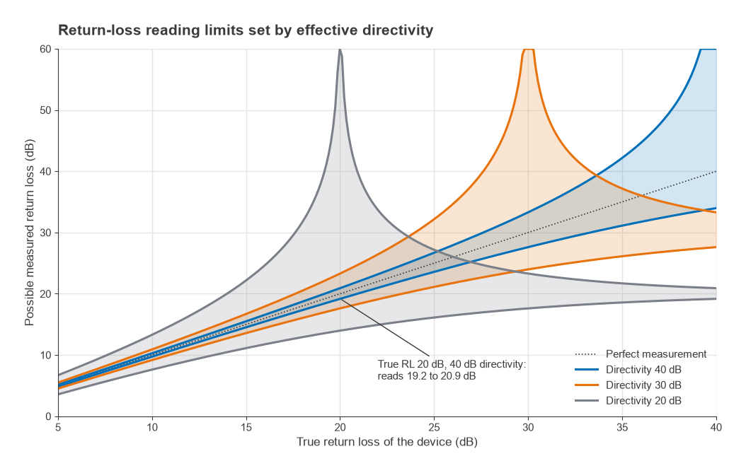
A coupler that leaks a little incident signal into the reflected-wave receiver makes every load look slightly mismatched. The residual leakage after calibration is the effective directivity, E_D. To a first approximation, ignoring source match and tracking errors, the measured reflection lies within

|Γ| − |E_D| ≤ |Γ_meas| ≤ |Γ| + |E_D|

For a device with a true return loss of 20 dB, |Γ| = 0.1. With 40 dB effective directivity, |E_D| = 0.01 and the reading lies between 19.2 dB and 20.9 dB. With 30 dB directivity the range widens to 17.6 dB to 23.3 dB. With 20 dB directivity, |E_D| equals |Γ| and the reading can be anywhere from 14.0 dB to a perfect-looking match. The practical rule is that a VNA cannot reliably measure return loss much better than its effective directivity, and the quality of the calibration standards largely sets that directivity.

Bounds on measured return loss versus true return loss for 20, 30 and 40 dB effective directivity — Figure 4: First-order reflection uncertainty from effective directivity alone. A true 20 dB return loss reads 19.2 to 20.9 dB with 40 dB directivity, but anywhere from 14.0 dB upward with 20 dB.

Low-Cost VNAs and Their Limits

Pocket VNAs such as the NanoVNA family have made network analysis affordable for students and hobbyists, and they are useful for antenna tuning, cable checks and filter alignment at lower frequencies. Their limits come from the hardware choices that make them cheap:

Dynamic range. Typically quoted around 60 to 70 dB in the lower bands for the original designs, falling substantially at higher frequencies, depending on hardware version and firmware. That is enough for a matching network but not for a deep filter stopband.
Harmonic operation. Some models reach their upper frequencies by using harmonics of a lower-frequency synthesizer, which reduces signal level and dynamic range in those bands.
Calibration standards. The supplied SOL standards are not characterized like a laboratory kit, so effective directivity and source match are worse, especially at higher frequencies.
Receiver architecture. Reduced receiver sets limit full two-port correction; many units measure S₁₁ and S₂₁ only and need the device reversed for the other parameters.
Connectors and stability. Small connectors wear quickly, and temperature drift is larger than on a laboratory instrument.

Used within these limits, and checked against a known reference, a low-cost VNA gives real engineering data. Results near the edge of its dynamic range, or return losses better than about 25 to 30 dB, deserve a check on a better instrument.

Frequently asked questions

What does a VNA measure?

A VNA measures the S-parameters of a device: the ratio of reflected and transmitted waves to the incident wave, in magnitude and phase, over frequency. From them it derives return loss, VSWR, impedance, gain, insertion loss, phase and group delay.

What is the difference between a VNA and a spectrum analyzer?

A VNA supplies its own stimulus and measures the device’s response to it, as ratios with phase. A spectrum analyzer has no built-in stimulus in its basic form and measures the absolute power of whatever signals arrive, at every frequency in its span. Use a VNA for linear network behaviour and a spectrum analyzer for spurs, harmonics, distortion and modulated signals.

What IF bandwidth should I use?

Start wide, around 1 kHz to 10 kHz, for fast sweeps while tuning. Narrow it to 100 Hz or less when measuring deep rejection or low-level signals, accepting the slower sweep.

Can a VNA measure noise figure?

Some VNAs offer noise figure measurement as an option, using either a noise source or the cold-source method. Otherwise a dedicated setup is used, as described in noise figure measurement.