

A MIMO system (multiple-input, multiple-output) uses several antennas at the transmitter and the receiver to get more out of a radio link than one antenna at each end can deliver. Multiple antennas offer three separate benefits: array gain raises the average SNR, diversity gain reduces deep fades, and multiplexing gain carries parallel data streams in the same bandwidth. A real design divides its antennas among these three, and the propagation channel decides how much of each is available.
This page sets out the antenna configurations and the three gains, with numbers for each. Two companion articles go deeper: beamforming covers steering energy with phased weights, and spatial multiplexing covers parallel streams. For the transceiver hardware behind them, see MIMO, Beamforming and Phased-Array Architectures.
SISO, SIMO, MISO and MIMO configurations
The names count the antennas seen by the channel. The “input” is the channel input, which is the transmitter, and the “output” is the receiver. A 2×4 link therefore has 2 transmit and 4 receive antennas. The table lists what each configuration can offer in ideal independent Rayleigh fading, with Nt transmit and Nr receive antennas.
| Configuration | Array gain | Diversity order | Parallel streams |
|---|---|---|---|
| SISO (1×1) | None | 1 | 1 |
| SIMO (1xNr) | Nr | Nr | 1 |
| MISO (Ntx1), no transmit CSI | None | Nt | 1 |
| MISO (Ntx1), with transmit CSI | Nt | Nt | 1 |
| MIMO (NtxNr) | Up to NtNr (one stream, CSI at both ends) | Up to NtNr | Up to min(Nt, Nr) |
The entries are upper limits and cannot all be reached at once. A link that sends the maximum number of streams spends its antennas on multiplexing and keeps little diversity. The formal statement of this is the diversity-multiplexing tradeoff, which says that a rate growing faster with SNR comes at the cost of a shallower outage slope.
Channel state information (CSI) is what the MISO row turns on. If the transmitter knows the channel, it can pre-rotate each antenna’s phase so the signals add in phase at the receiver. If it does not, it can only spread power across antennas with a code.
Array gain
Array gain is the rise in average SNR from coherent combining. Signal voltages from N antennas add in phase, so signal power grows as N2, while independent noise from N receive chains adds in power and grows as N. The net SNR gain is:
GA = 10 log10(N) dB
Four receive antennas give 6.02 dB, two give 3.01 dB and eight give 9.03 dB. This gain exists even without fading, because it comes from collecting more signal. In a link budget, 6 dB of array gain can be spent as extra range, lower transmit power or a higher-order modulation. It assumes that each chain has its own noise and that the combiner knows the channel phases. On transmit with fixed total power, the same 10 log10(N) applies, provided the transmitter has CSI or a known direction.
Diversity gain and receive combining
Diversity gain is a different effect: it changes the slope of the error or outage curve, not simply its position. Multipath fading causes the occasional deep fade, and if each antenna fades independently, all of them fading together is far less likely than any one fading. The diversity order L is the number of independent fading branches, and at high SNR outage falls by a decade for every 10/L dB of added SNR.
Maximal ratio combining versus selection
Maximal ratio combining (MRC) weights each branch by the conjugate of its channel, which aligns phases and favours strong branches. Its output SNR is the sum of the branch SNRs. Selection combining simply picks the strongest branch and needs only one receive chain after an RF switch. For L independent Rayleigh branches with mean SNR γ̄ per branch and threshold γth, writing x = γth/γ̄:
Pout,MRC = 1 – e-x Σk=0L-1 xk/k!
Pout,SC = (1 – e-x)L
Worked example: outage with 1, 2 and 4 branches
Take a receiver that needs 5 dB SNR on a link with a mean SNR of 15 dB per branch. The ratio is x = 10-1 = 0.1.
| Receiver | Outage probability | About one fade in |
|---|---|---|
| Single antenna | 0.0952 | 11 |
| 2-branch selection | 0.00906 | 110 |
| 2-branch MRC | 0.00468 | 214 |
| 4-branch MRC | 3.85 x 10⁻⁶ | 260,000 |
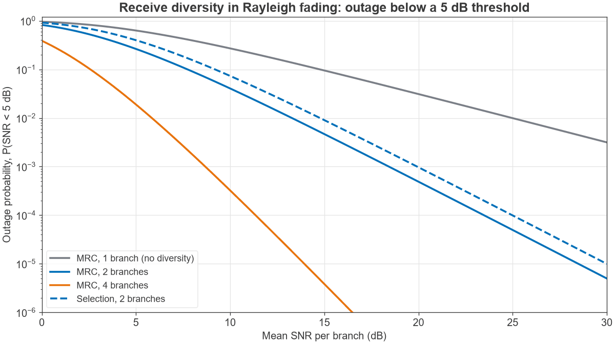
A Monte Carlo run of 4 million Rayleigh draws returned 0.0953 and 0.00470 for the one- and two-branch MRC cases. The four-branch result is from the closed form alone, because too few outage events occurred in that run to confirm it. Going from one branch to two improves outage by about 20 times, far more than the 3 dB of array gain would suggest alone. Figure 1 shows the change in slope.
Transmit diversity without CSI
With two transmit antennas and no CSI, the Alamouti space-time block code achieves diversity order 2 at one symbol per symbol period. Because total power is shared across two antennas, it performs 3.01 dB worse than 2-branch receive MRC with the same diversity order. That difference is exactly the missing array gain. Alamouti coding sends one stream’s worth of data, so it is a diversity method and not spatial multiplexing.
MIMO capacity and multiplexing gain
With a rich scattering channel, MIMO provides several spatial paths in the same bandwidth. With no CSI at the transmitter and power shared equally, the capacity of a channel matrix H at SNR ρ is:
C = log2 det(I + (ρ/Nt) H HH) b/s/Hz
For fading channels the ergodic capacity is the average of this over the channel distribution. At high SNR, capacity rises by about min(Nt, Nr) b/s/Hz for each 3 dB of SNR, compared with 1 b/s/Hz per 3 dB for SISO. This slope is the multiplexing gain. SNR and Eb/N0 set the starting point on these curves.
Worked example: capacity at 20 dB SNR
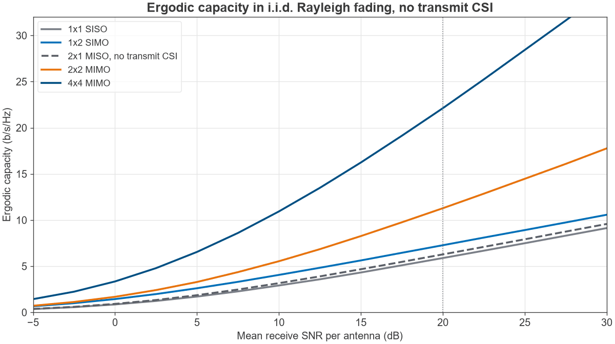
The table gives ergodic capacity in i.i.d. Rayleigh fading at 20 dB mean receive SNR per antenna, averaged over 200,000 channel draws, with the rate for 20 MHz of bandwidth. For reference, a non-fading AWGN channel at the same SNR gives 6.66 b/s/Hz. The Monte Carlo 1×1 value of 5.88 agrees with the exact integral, 5.884 b/s/Hz.
| Configuration | Ergodic capacity (b/s/Hz) | Rate in 20 MHz (Mb/s) |
|---|---|---|
| 1×1 SISO | 5.88 | 118 |
| 2×1 MISO, no CSI | 6.28 | 126 |
| 1×2 SIMO | 7.27 | 145 |
| 2×2 MIMO | 11.29 | 226 |
| 4×4 MIMO | 22.14 | 443 |
Compare the 1×2 and 2×1 rows. Both have two antennas and the same diversity order, but the receive side adds array gain and the transmit side without CSI does not. Moving to 2×2 nearly doubles the SISO figure, and 4×4 nearly quadruples it. These are theoretical limits under ideal assumptions: independent fading, perfect receiver channel knowledge and no hardware impairments. Practical rates will be lower.
Antenna spacing and correlation
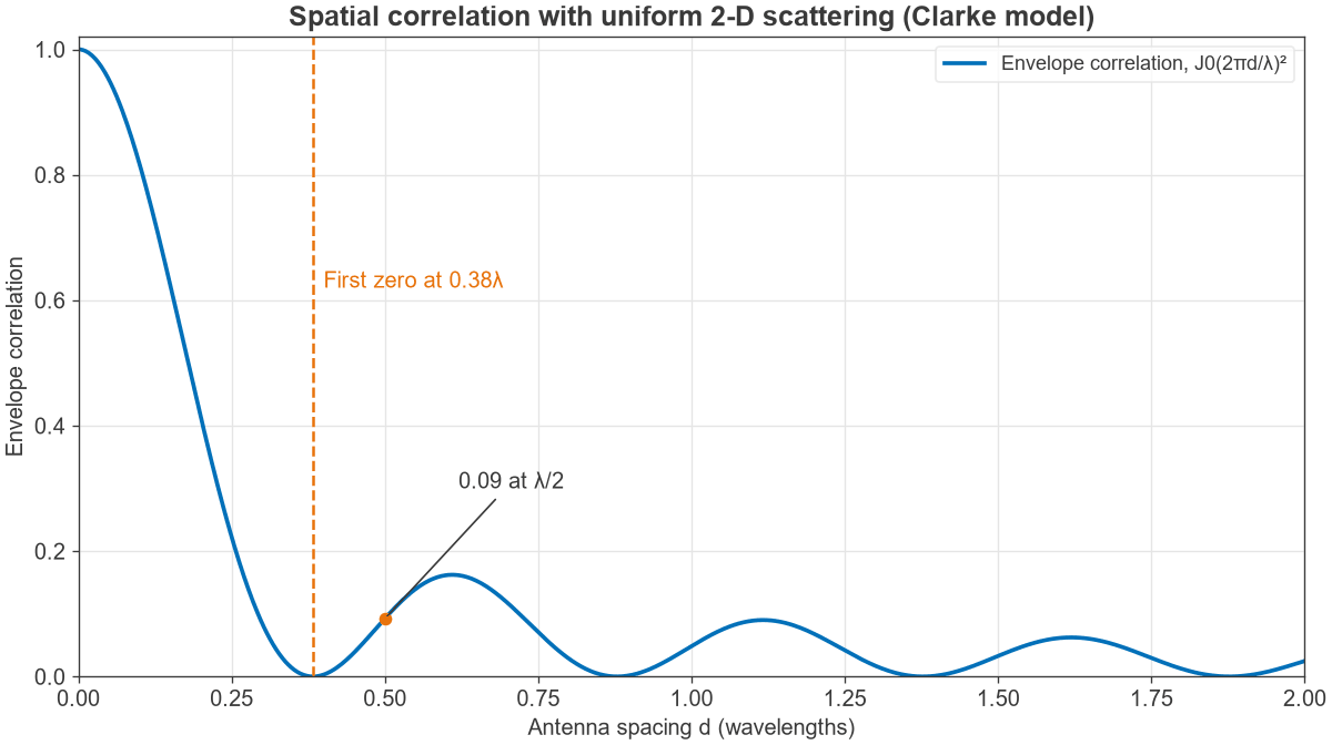
Every figure above assumes independent fading at each antenna, and real antennas are not independent. For a uniform ring of scatterers around vertically polarised antennas (the Clarke model), the envelope correlation between two antennas at spacing d is approximately:
ρe ≈ J0(2πd/λ)2
The first zero is at 0.38λ, and at half a wavelength the correlation is 0.09, as Figure 3 shows. At 3.5 GHz, where λ = 85.7 mm, half-wavelength spacing is 42.8 mm. At 2.4 GHz, λ = 124.9 mm and half-wavelength spacing is 62.5 mm. Fitting those spacings into a handset or small IoT product is often the limiting design problem.
Moderate correlation is tolerable. In the outage example above, 2-branch MRC with an envelope correlation of 0.5 gives an outage of 0.00878 against 0.00468 for independent branches. That is close to the result for uncorrelated selection combining, but much better than a single antenna at 0.0952.
The Clarke result assumes scattering from all directions. A base station on a tower sees a narrow angular spread, and may need several wavelengths to ten or more between antennas for low correlation. Dual-polarised antennas are the common alternative, because orthogonal polarisations decorrelate within a single antenna footprint.
RF design considerations
The antenna count sets a hardware bill. Each digital branch needs its own PA, LNA, filters, mixers and data converters, so 4×4 costs roughly four times the RF chain power of SISO. The specific points to watch are:
- Mutual coupling. Closely spaced antennas load each other, which reduces efficiency and shifts the match. See antenna parameters for how efficiency and gain are defined.
- Envelope correlation from S-parameters. For lossless antennas, envelope correlation can be estimated from a two-port measurement. For real, lossy antennas it should be measured from far-field patterns, as described under measuring radio performance.
- Branch imbalance. One weak antenna reduces both diversity and rank. A hand on a phone can do this.
- Chain matching. Coherent combining needs a known phase between chains, so branches usually share an LO and are calibrated. TDD systems that infer the downlink from the uplink also need calibrated transmit and receive paths.
Choosing how to use the antennas
| Link condition | Best use | Reason |
|---|---|---|
| Low SNR, cell edge | Beamforming or receive combining | Power gain is worth more than extra streams |
| High SNR, rich scattering | Spatial multiplexing | Capacity grows with the number of streams |
| Fading dominates, CSI poor or fast-changing | Diversity coding | Needs no feedback from the receiver |
| Line of sight, directional | Beamforming | The channel usually supports few streams |
Modern radios change this choice continually, adapting the rank and the precoder to channel reports. The general guide is that streams pay at high SNR and power gain pays at low SNR. Antennas and propagation for radio designers describes the channels that drive this decision.
Frequently asked questions
What is the difference between MIMO and beamforming?
MIMO is the general case of multiple antennas at both ends. Beamforming is one way to use them, applying phase and amplitude weights so that one signal adds constructively in a chosen direction. A MIMO link may beamform a single stream, send several streams, or do both.
Does MIMO increase range or speed?
It can do either, but not fully at once. Array and diversity gain improve the link margin, which extends range or reliability. Multiplexing raises peak rate, and it needs enough SNR and channel rank to work. At the cell edge a system usually gives up streams for power gain.
How far apart should MIMO antennas be?
Half a wavelength is the usual starting point, and it gives an envelope correlation of about 0.09 in the idealised Clarke model. A base station with low angular spread needs much more spacing, while dual polarisation provides a useful second branch at almost no spacing at all.
Do both ends need the same number of antennas?
No. The stream count is limited by the smaller of the two antenna counts, and extra antennas on either side still provide array gain and diversity. A 4×2 link carries at most two streams but has spare spatial degrees of freedom for beamforming.
Related topics
For the two main techniques, read beamforming and spatial multiplexing. MIMO, Beamforming and Phased-Array Architectures covers transceiver structures, and Antennas and Propagation for RF Designers covers the antenna side. Both sit within the wider radio architectures series.