

Part 6 traced the transmit chain from baseband samples to the antenna and ended at the power amplifier. The PA is usually the largest single consumer of DC power in a radio, the main source of in-band and adjacent-channel distortion, and the component that sets the thermal design. In a base station it can account for most of the electricity bill for the radio unit; in a handset it is a large share of the battery drain while transmitting.
This part covers how PAs are classified, what efficiency each class can reach in theory, and why practical transmitters rarely get near those numbers. The short answer to the last question is back-off: modern signals have high peak-to-average ratios, and a PA biased for linearity spends most of its time far below the power level where it is efficient.
Measuring Efficiency
Two definitions are in common use. Drain efficiency (collector efficiency for bipolar devices) is the RF output power divided by the DC supply power:
ηD = Pout / PDC
Power-added efficiency (PAE) subtracts the RF drive power, which matters when the stage gain is low:
PAE = (Pout − Pin) / PDC = ηD (1 − 1/G)
where G is the linear power gain. With 20 dB of gain the difference between the two is only 1%. With 10 dB it is 10% of the drain efficiency figure, and for a high-frequency stage with 6 dB of gain, a quarter of the output power came from the driver. Whatever is not delivered as RF becomes heat: Pdiss = PDC + Pin − Pout.
Conduction Angle: Classes A, AB, B and C
The classic linear-mode classes are distinguished by bias point, which determines the conduction angle: the fraction of each RF cycle, in degrees, during which the transistor conducts. The device behaves as a controlled current source in every case; only the portion of the cycle it spends conducting changes.
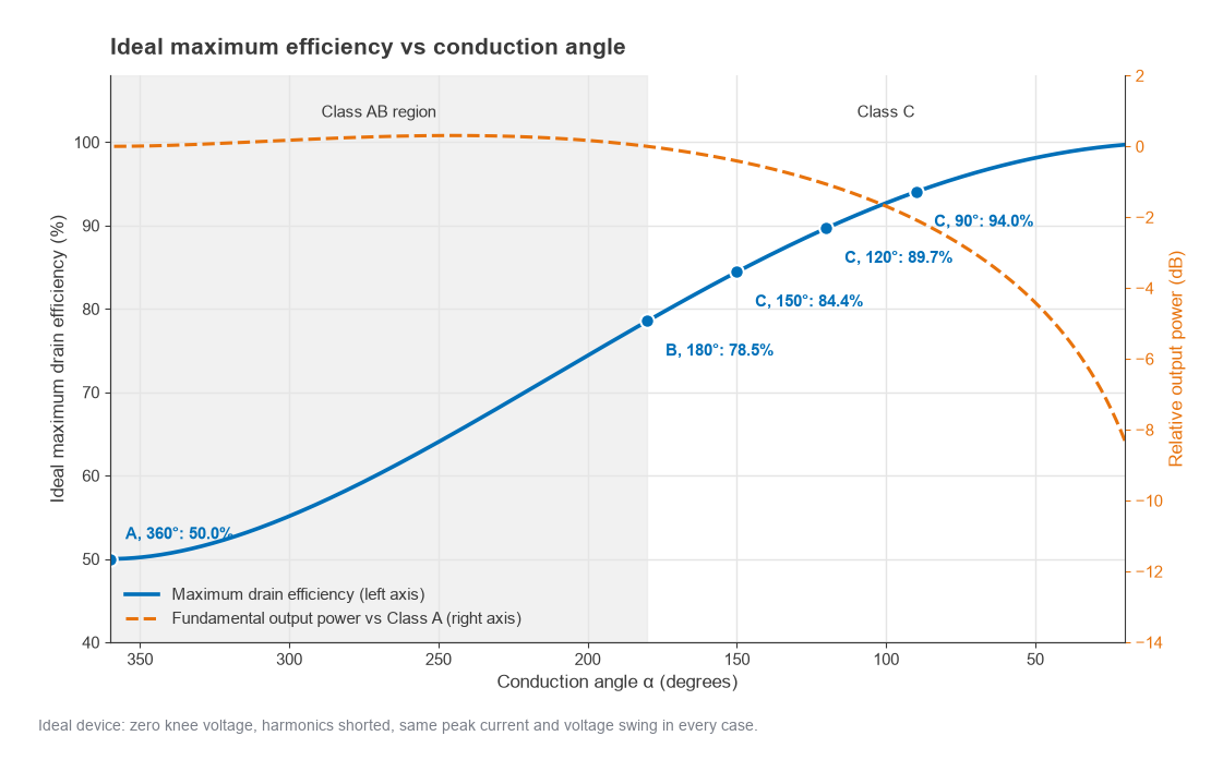
- Class A is biased at the middle of its current range and conducts for the full 360°. It is the most linear but wastes the most power, since full bias current flows even with no signal.
- Class B is biased at cutoff and conducts for 180°. A single device produces a half-wave rectified current; the tuned output network restores a sinusoidal voltage. Push-pull pairs cover both halves.
- Class AB lies between, with a small quiescent current and conduction angle between 180° and 360°. Almost all linear communications PAs operate here, because pure Class B suffers crossover distortion near cutoff.
- Class C is biased below cutoff and conducts for less than 180°. Efficiency rises, but output power and gain fall, and the output amplitude no longer tracks the input linearly. It suits constant-envelope signals such as FM.
For an ideal device with zero knee voltage, a harmonically shorted load and a conduction angle α (in radians), the maximum drain efficiency is
η = (α − sin α) / { 4 [ sin(α/2) − (α/2) cos(α/2) ] }
At α = 2π the sine terms vanish and cos(π) = −1, giving 2π / 4π = 50%, the Class A limit. At α = π, sin(π/2) = 1 and cos(π/2) = 0, giving π/4 = 78.5%, the Class B limit. The table lists a few more points.
| Class | Conduction angle | Ideal maximum efficiency | Linearity |
|---|---|---|---|
| A | 360° | 50.0% | Best |
| AB | 180° to 360° | 50.0% to 78.5% | Good, with care at low current |
| B | 180° | 78.5% | Crossover distortion if single-ended near cutoff |
| C | 150° | 84.4% | Poor amplitude linearity |
| C | 120° | 89.7% | Poor amplitude linearity |
| C | 90° | 94.0% | Poor; low output power and gain |
Efficiency approaches 100% as the conduction angle approaches zero, but the fundamental output current approaches zero too, so the device delivers vanishing power. Practical Class C designs settle somewhere around 120° to 150°.
Switching Amplifiers: Classes D, E and F
A different route to high efficiency is to stop treating the transistor as a current source and run it as a switch. An ideal switch has either zero voltage across it or zero current through it, so it dissipates nothing. The output network shapes the voltage and current waveforms so that they do not overlap.
Class D uses two switches, in a half-bridge or full-bridge, to produce a square voltage wave that a series-tuned filter converts to a sinusoid. Ideal efficiency is 100%. At RF the device output capacitance is the limit: every cycle the capacitance is charged to the supply voltage and then discharged through a switch, dissipating roughly C V2 f in total, a loss that grows in proportion to frequency.
Class E uses a single switch with a load network designed so that, at the moment the switch closes, the voltage across it is zero and its slope is zero. This zero-voltage switching absorbs the device output capacitance into the network and avoids the C V2 f loss. Class E is popular from HF up through the low microwave range. Its drawback is a high peak drain voltage, about 3.6 times the supply for the classic design, which constrains the supply voltage relative to device breakdown.
Class F works with a current-source device but controls the harmonic terminations. Presenting short circuits at even harmonics and open circuits at odd harmonics squares up the drain voltage while the current stays half-sinusoidal, reducing their overlap. Efficiency approaches 100% as more harmonics are controlled; in practice the second and third harmonics are terminated and the rest are left to the device capacitance. Inverse Class F swaps the even and odd terminations.
Switching and harmonically tuned amplifiers are nonlinear in amplitude. They are used directly for constant-envelope signals, or as the efficient core inside polar, envelope-tracking and outphasing transmitters described in Part 6.
Worked Example: Load Line, Efficiency and Heat
Consider a Class B stage (a reasonable first approximation to deep Class AB) intended to deliver 40 W at its peak, from a 28 V supply, using a device with a knee voltage of 3 V.
Optimum Load
The usable peak voltage swing is VDD − Vknee = 25 V. The load resistance that lets the device reach both full voltage and full current swing at the target power is
Ropt = (VDD − Vknee)2 / (2 Pout) = 252 / 80 = 7.81 Ω
This is a power match, not a conjugate match, and it is well below 50 Ω. Transforming 7.81 Ω to 50 Ω with a single L-section requires a loaded Q of √(50/7.81 − 1) = √5.40 ≈ 2.32, which is comfortable. Higher-power devices have lower optimum loads and need multi-section matching to keep bandwidth.
Currents and Efficiency at Peak Power
The fundamental current amplitude is I1 = 2Pout / Vpk = 80 / 25 = 3.2 A. For a half-sine Class B current, the fundamental is half the peak, so Imax = 6.4 A, and the DC component is Imax/π = 2.04 A. The DC input power is 28 × 2.04 = 57.0 W, so
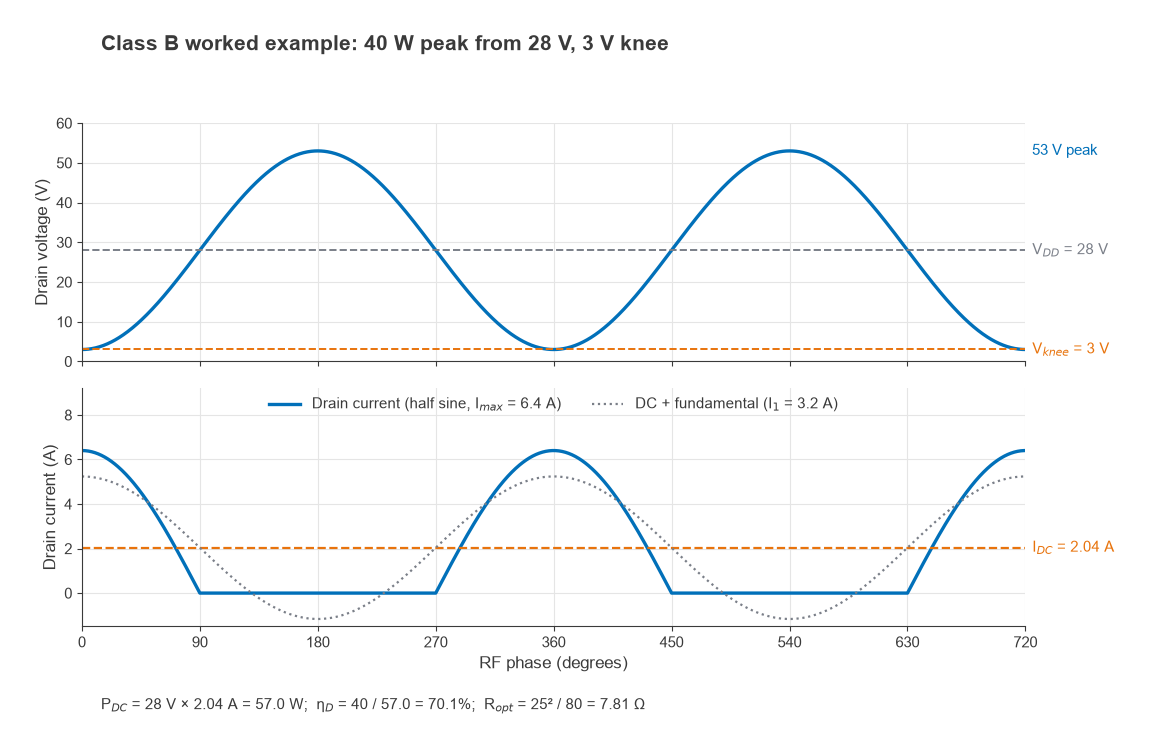
ηD = 40 / 57.0 = 70.1%
This agrees with the shortcut η = (π/4)(Vpk/VDD) = 0.785 × 25/28 = 70.1%. The knee voltage alone has cost more than 8 percentage points.
If the stage has 15 dB of gain, the drive power is 40 / 31.6 = 1.26 W, and
PAE = (40 − 1.26) / 57.0 = 67.9%
Dissipation is 57.0 + 1.26 − 40 = 18.3 W. With a junction-to-case thermal resistance of 1.2 °C/W and a flange held at 85 °C, the junction runs at 85 + 1.2 × 18.3 ≈ 107 °C.
The Same Stage at 8 dB Back-Off
Now drive the amplifier with a modulated signal whose average power sits 8 dB below the 40 W peak, or 6.34 W. In Class B the DC current is proportional to the output voltage amplitude, so efficiency scales with the square root of output power relative to peak:
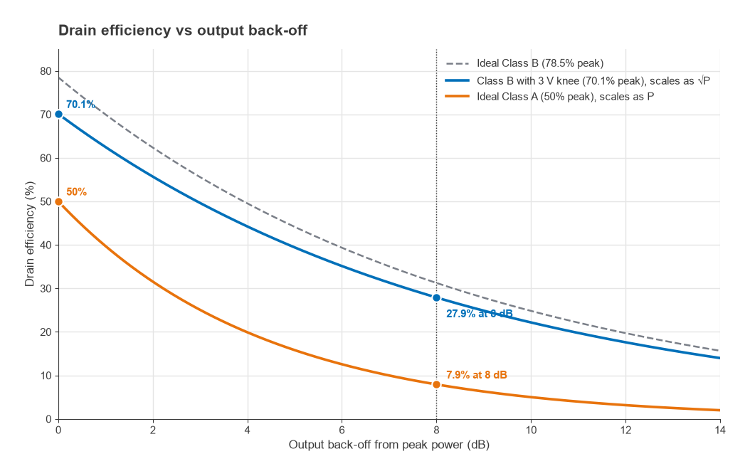
η = ηmax √(Pout/Pmax) = 70.1% × √(6.34/40) = 70.1% × 0.398 ≈ 27.9%
The DC power is 6.34 / 0.279 = 22.7 W, and the dissipation (ignoring drive) is about 16.4 W. Output power fell by a factor of 6.3, yet the heat to be removed fell by less than 2 W. For a Class A stage the picture is worse, because efficiency scales linearly with output power: an ideal 50% Class A amplifier is only about 7.9% efficient at 8 dB back-off.
Why Back-Off Dominates Real Efficiency
Single-carrier QPSK had modest envelope variation. OFDM, multicarrier and spread-spectrum signals are different: their envelopes approach a Rayleigh distribution, with occasional peaks 10 dB or more above the average. Crest factor reduction (CFR) clips and filters these peaks digitally, typically bringing the PAPR to somewhere around 7 to 8 dB with an acceptable EVM penalty. The PA must still pass those peaks without heavy compression, so its average operating point sits that far below saturation.
The efficiency that matters is therefore the average over the signal’s amplitude distribution, not the peak figure on the data sheet. The square-root law of Class B and the linear law of Class A show why conventional amplifiers do poorly here. Three families of solutions follow:
- Reduce the required back-off by making the PA more linear near saturation, which is the job of digital predistortion.
- Change the load as the envelope changes, so the PA stays near its peak efficiency over a range of powers. This is the Doherty principle.
- Change the supply as the envelope changes, which is envelope tracking.
Device technology sets the starting point. Gallium nitride (GaN) HEMTs on silicon carbide dominate high-power infrastructure because of their high breakdown voltage, power density and good efficiency at gigahertz frequencies. Silicon LDMOS remains common below about 3 GHz, where it is mature and low in cost. Handset PAs are mostly GaAs HBTs. Each technology has its own knee voltage, output capacitance and thermal behavior, all of which shift the numbers in the example above.
Next in the Series
Part 8, PA Linearization (Feedforward, DPD, Doherty), covers the techniques that let a PA run closer to saturation without breaking its spectral mask: feedforward cancellation, digital predistortion with memory, and the Doherty amplifier’s load modulation, together with a worked comparison of the DC power each approach saves.