

RF fundamentals are the units, wave properties and component behaviours that every later topic in RF design depends on: decibels and dBm, the link between frequency and wavelength, power, Q factor, skin effect and the parasitics of real components. They explain why circuits that work at audio frequencies stop behaving as drawn once the wavelength approaches the size of the hardware.
This hub introduces each of those ideas briefly and links to the detailed page for each one. It is the first section of the RF design guide, and most readers new to the subject should work through it before moving on to transmission lines, S-parameters and noise.
Why Lumped Models Fail at RF
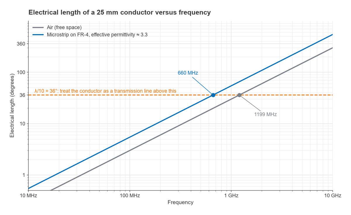
Ordinary circuit analysis treats every wire as an equipotential node and every component as its ideal symbol. Both assumptions rely on the circuit being electrically small, meaning that a signal crosses it in a tiny fraction of one cycle. The relevant measure is electrical length, the physical length expressed as a fraction of the guided wavelength:
θ = 360° × ℓ / λg, with λg = c / (f √εeff)
A common rule of thumb says that once a conductor exceeds about λ/10, or 36° of electrical length, it should be modelled as a transmission line. Take a 25 mm trace. In air it reaches λ/10 at about 1.2 GHz. As a microstrip on FR-4, with an effective permittivity of roughly 3.3, the wave travels about 1.8 times more slowly and the same trace reaches λ/10 at about 660 MHz. At 2.4 GHz the trace is about 131° long, more than a third of a wavelength, and its input impedance depends strongly on what terminates it.
Parasitics inside components
The same scaling applies inside components. Capacitors have series inductance, inductors have winding capacitance, and resistors have both. A 100 pF capacitor with 0.5 nH of equivalent series inductance resonates at f = 1/(2π√(LC)) ≈ 712 MHz. Below that frequency it behaves as a capacitor; above it, as an inductor. A designer who chooses that part to decouple a 2.4 GHz supply is in fact placing about 7 Ω of inductive reactance in the path.
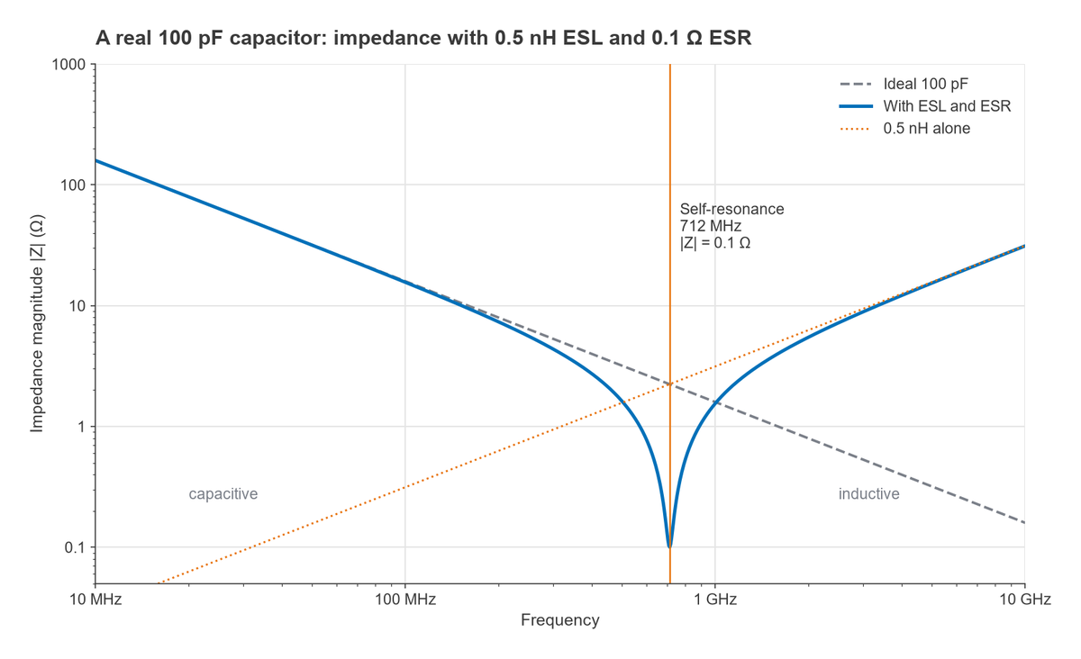
Those two observations, distributed lines and component parasitics, are the reason RF design has its own toolset of matched impedances, S-parameters and the Smith chart. The transmission lines and impedance matching section picks up where this one ends.
Topics in This Section
Units and power
- dB, dBm, dBW and dBc Explained: logarithmic units, conversion between dBm and watts, voltage versus power decibels, and a converter.
- Power in RF Systems: Average, Peak and PEP: how average, peak and peak envelope power are defined and measured.
Waves and spectrum
- Frequency and Wavelength in RF Design: λ = c/f, guided wavelength and why physical size matters.
- RF Frequency Bands and Designations: the ITU bands from VLF to EHF and the common letter-band names.
- Properties of Electromagnetic Waves: fields, polarization, impedance of free space and propagation.
Real components at RF
- Q Factor in RF Circuits: component Q, loaded and unloaded Q, and bandwidth of resonant circuits.
- Skin Effect and Conductor Loss at RF: why current crowds to the surface and how that raises resistance.
- Parasitics of Passive Components at RF: equivalent circuits of capacitors, inductors and resistors, and self-resonance.
Three Quantities to Learn First
Decibels
RF signals span enormous ranges of power. A transmitter may put out 1 W while the receiver at the other end of the link sees 10−13 W. Decibels compress that range into numbers that add and subtract: 1 W is +30 dBm and 10−13 W is −100 dBm, a difference of 130 dB. Gains and losses through a chain are then summed rather than multiplied.
Q factor
Q compares the energy stored in a component or resonator with the energy lost per cycle. For a series inductor model, Q = X/R = 2πfL/R. A 10 nH inductor with 0.5 Ω of series resistance at 1 GHz has X = 62.8 Ω and Q ≈ 126. Component Q sets the insertion loss of matching networks and filters and the phase noise of oscillators.
Skin depth
At high frequency, current flows in a thin layer near the conductor surface. The skin depth is δ = √(ρ / (π f μ)). For copper, with ρ ≈ 1.68 × 10⁻⁸ Ω·m, δ is about 65 µm at 1 MHz and about 2.1 µm at 1 GHz. Once δ is much smaller than the conductor thickness, resistance rises roughly with √f, and surface roughness on PCB copper starts to matter.
A Suggested Order
Students should start with decibels and frequency and wavelength, because every later page uses them. Power definitions come next, followed by Q factor, skin effect and parasitics, which explain most of the surprises met on a first RF board. From there the natural path leads to transmission lines, then S-parameters, then noise in RF systems. Readers who prefer a single long overview can also use the earlier article Mastering RF Engineering Fundamentals.
Frequently Asked Questions
What are the basics of RF?
The basics are the decibel units used to describe power and gain, the relationship between frequency and wavelength, how RF power is defined, and how real components and conductors behave at high frequency. Together they explain when a circuit must be treated as a set of transmission lines rather than ideal wires.
What should I learn first in RF engineering?
Learn decibels and dBm first, then wavelength and electrical length, then transmission lines and impedance matching. With those in place, S-parameters, noise figure and linearity become straightforward, and the Radio Architectures series shows how they combine in a complete radio.
At what frequency does a circuit become an RF circuit?
There is no single frequency. The question is whether any conductor or component is a significant fraction of a wavelength, with λ/10 as a common threshold. A 25 mm FR-4 trace crosses that line near 660 MHz, while a 1 m cable crosses it near 30 MHz in air.
Related Topics
Continue with transmission lines, the Smith chart and S-parameters. Unfamiliar terms are defined in the RF and wireless glossary.