

Part 13, Direct RF Sampling and Software-Defined Radio, ended with the observation that even a radio that digitizes at RF still needs analog hardware between the antenna and the converter. That hardware has to select the band, set the noise figure, keep strong signals out of the receiver and route the transmitter’s output to the antenna with as little loss as possible.
In a handset or small radio, that hardware is usually packaged as a front-end module (FEM). This part looks at what goes into a module, how duplexers and switches separate transmit from receive, and how their loss, isolation and linearity enter the system budget. The filter technologies themselves were covered in Part 9, RF Filters; here the concern is how they are used.
What a Front-End Module Contains
The term covers a range of integration levels. At the simple end, a module might combine a PA and a transmit/receive switch for a Wi-Fi or short-range radio. At the complex end, a cellular module for a group of bands can contain:
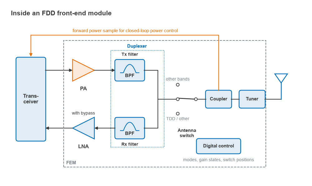
- One or more power amplifiers, with their bias and control circuits.
- Low-noise amplifiers, sometimes with bypass modes for strong-signal conditions.
- Duplexers or multiplexers for FDD bands, and bandpass filters for TDD bands.
- Band-select and antenna switches.
- A directional coupler that samples the transmitted power for closed-loop power control.
- Impedance matching networks and, in some designs, an antenna tuner.
- A digital control interface for setting modes, gain states and switch positions.
Integration shortens interconnects and removes board-level matching, which reduces loss between components. It also lets the module vendor characterize the PA into the actual filter impedance rather than into 50 Ω, which matters because an acoustic filter’s input impedance varies across its passband. The downside for the system designer is reduced visibility: the module’s specifications at its ports are what the system budget has to work with.
Duplexers and FDD Isolation
In frequency-division duplex, the transmitter and receiver operate simultaneously on different frequencies and share an antenna. A duplexer is two bandpass filters, one for each band, joined at a common antenna port through a matching network that makes each filter look like an open circuit in the other’s band. Its key specifications are insertion loss in each path and isolation between the transmit and receive ports, measured both in the transmit band and in the receive band.
Those two isolation figures address different problems. Isolation in the transmit band keeps the transmitter’s carrier from overloading the LNA or generating intermodulation and, in a zero-IF receiver, second-order products (see Part 12). Isolation in the receive band keeps the transmitter’s broadband noise, which extends into the receive band, from raising the receiver’s noise floor. The receive filter cannot help with the second problem, because the noise is at the same frequency as the wanted signal. It must be removed by the transmit filter before it reaches the antenna port.
Worked example: how much isolation?
Assume the PA output carries a noise density of −130 dBm/Hz in the receive band, and the receiver has a noise figure of 3 dB referred to the duplexer’s receive port. The receiver’s own noise floor at that port is −174 + 3 = −171 dBm/Hz.
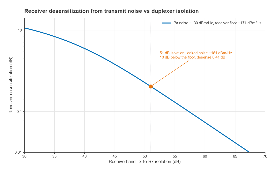
- Allowing the leaked transmit noise to sit 10 dB below the receiver floor means it must be at or below −181 dBm/Hz.
- Required receive-band isolation: −130 − (−181) = 51 dB.
- The resulting desensitization is 10log(1 + 10−1) = 0.41 dB.
Now the transmit-band case. With +27 dBm at the PA output and 55 dB of transmit-band isolation, the carrier reaches the LNA input at +27 − 55 = −28 dBm. That level has to sit comfortably below the LNA’s input compression point, and the receiver’s IIP2 and IIP3 must be good enough that this signal, combined with any external blocker, does not create products in the receive channel. If either isolation figure cannot be achieved in a single acoustic duplexer, the alternatives are a higher-order filter, additional filtering between PA and duplexer, or reduced PA output noise, often by moving filtering earlier in the transmit chain as Part 11 suggested.
Closely spaced bands make all of this harder. When the duplex gap between transmit and receive is a small fraction of the carrier frequency, the filter skirts must be very steep, which pushes designs towards high-Q BAW or temperature-compensated SAW resonators. Carrier aggregation adds more filters to the same antenna port. A quadplexer or hexaplexer must keep each filter’s passband unloaded by all the others, and the insertion loss rises as filters are added.
Insertion Loss and What It Costs
Every decibel of loss between the antenna and the LNA adds directly to the receiver noise figure. A passive, matched component at the reference temperature has a noise factor equal to its loss, F = L. Using the Friis equation from Part 4, a lossy element followed by an LNA gives
Ftotal = L + (FLNA − 1) × L = L × FLNA
In decibels the losses simply add. A duplexer with 2 dB receive-path loss in front of an LNA with a 1.5 dB noise figure produces a 3.5 dB system noise figure before any later stage is considered. Add 0.5 dB for an antenna switch and the front end is at 4 dB. This is why the LNA is placed as close to the antenna as the architecture allows, and why switch and filter loss receive so much attention.
On the transmit side, loss after the PA costs power and efficiency. To deliver +24 dBm at the antenna through 2 dB of duplexer loss and 0.5 dB of switch loss, the PA must produce +26.5 dBm. In linear terms that is 447 mW instead of 251 mW, and the extra 196 mW is dissipated as heat in the filter. Since PA efficiency (Part 7) is never 100%, the supply power increases by more than that: at 40% efficiency the DC input grows by about 490 mW. Heating in acoustic filters also shifts their frequency response with temperature, which is a further reason to keep transmit-path loss low.
Switches: Loss, Isolation and Linearity
TDD radios use a transmit/receive switch instead of a duplexer, since transmission and reception do not overlap in time. Multi-band radios use further switches to select among filters and antennas. Most modern RF switches are built on silicon-on-insulator CMOS, with stacked transistors to divide the RF voltage across several devices when the switch is off. GaAs pHEMT and PIN diode switches remain in use for some higher-power or higher-frequency applications.
| Specification | What it affects |
|---|---|
| Insertion loss | Receive noise figure and transmit power, as above |
| Isolation | Leakage between ports, including PA power reaching an idle LNA in TDD |
| Power handling (P0.1dB or P1dB) | Compression of the transmit signal at high power |
| Harmonics and IMD | Spurious emissions and intermodulation with co-located radios |
| Switching time | TDD guard periods and fast band changes |
Switch linearity is easy to overlook because the device is “passive.” An SOI switch handling +30 dBm sees a peak RF voltage of 10 V in a 50 Ω system (Vpk = √(2 × 1 W × 50 Ω)), more under mismatch, divided across its stack of off-state transistors, and the nonlinear capacitance of those devices generates harmonics and intermodulation. When two transmitters share an antenna path, for example in carrier aggregation, or when a strong external signal arrives at the antenna during transmission, the switch can produce third-order products that land in a receive band. The intercept analysis from Part 3 applies to switches and filters just as it does to amplifiers.
Mismatch, Antenna Tuning and the Coupler
The front end is designed for 50 Ω, but a handset antenna’s impedance changes with frequency and with the user’s hand and head. Mismatch reflects power. For a reflection coefficient |Γ|, the return loss is −20log|Γ| and the mismatch loss is −10log(1 − |Γ|2).
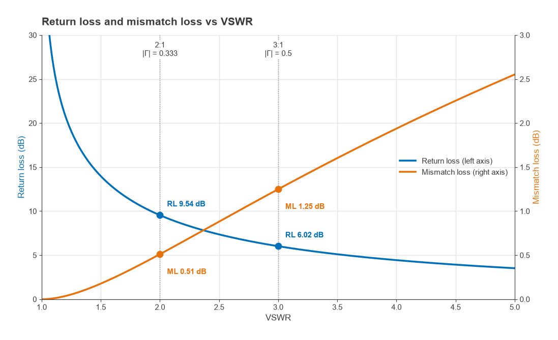
At a VSWR of 2:1, |Γ| = (2 − 1)/(2 + 1) = 1/3. The return loss is 20log(3) = 9.54 dB, and the mismatch loss is −10log(1 − 1/9) = 0.51 dB. At 3:1, |Γ| = 0.5, the return loss is 6.02 dB and the mismatch loss is 1.25 dB. The power figures understate the real problem: a PA designed for 50 Ω and presented with a mismatched load may lose output power, efficiency and linearity by more than the mismatch loss alone, and duplexer responses distort when their ports are not terminated correctly.
Antenna tuners address this with switched or variable capacitors that re-match the antenna across bands and use cases. The directional coupler at the module output samples forward (and sometimes reflected) power so the transceiver can regulate output power in a closed loop. Coupler directivity limits how accurately the forward power is measured under mismatch, since a fraction of the reflected wave leaks into the forward port.
Next in the Series
With the transmitter, receiver and front end all described, the remaining task is to tie them to the path between two antennas. Part 15, Link Budgets, Putting the Radio Together, works through transmit power, antenna gain, path loss, noise figure and required SNR to show how much margin a link really has.