

Part 8 showed how digital predistortion and the Doherty amplifier keep a PA’s adjacent-channel emissions under control while preserving efficiency. Linearization works close to the carrier. It does nothing for harmonics, for broadband noise that falls in a co-located receiver’s band, or for strong signals arriving at the receiver from other transmitters. Those problems are handled by filters, which appear at almost every stage of both the transmit and receive chains.
Earlier parts treated filters as boxes with a passband and some rejection. The image filter in the superheterodyne receiver of Part 2, the preselector ahead of the LNA in Part 4 and the anti-aliasing filter of Part 5 all assumed a filter could be built to order. This part looks at what actually limits a filter and which technology suits which job.
Filter Specifications
A filter specification normally includes the following:
- Insertion loss in the passband, in dB. Ahead of an LNA it adds directly to the noise figure. After a PA it wastes output power and turns into heat in the filter.
- Passband ripple and return loss, which affect EVM and the match presented to adjacent stages.
- Rejection at specified frequencies, such as the image, the LO, the opposite duplex band or a harmonic.
- Group delay variation across the passband. Sharp skirts come with large delay peaks near the band edges, which distort wideband modulated signals.
- Power handling and, for transmit filters, passive intermodulation.
- Temperature coefficient of frequency (TCF), which shifts the passband with temperature and eats into guard bands.
Several of these pull against one another. More resonators give steeper skirts but more loss and more group delay variation. A narrower fractional bandwidth gives better selectivity but, for a given resonator quality, higher loss.
Resonator Q and Insertion Loss
The unloaded quality factor Qu of the resonators is the single parameter that most separates filter technologies. For a coupled-resonator bandpass filter derived from a lowpass prototype with element values g1 to gn, the midband insertion loss due to finite Q is approximately
IL ≈ 4.343 × (f0 / BW) × Σ gk / Qu dB
where f0 is the center frequency and BW the passband bandwidth. The equation says three things. Loss rises in proportion to the number and size of the prototype elements, which grow with filter order and ripple. Loss is inversely proportional to fractional bandwidth, so a 1% filter has ten times the loss of a 10% filter with the same resonators. And loss is inversely proportional to Qu, which is set by the technology.
The order needed for a given rejection follows from the prototype response. For a Chebyshev response with passband ripple Ar dB, the attenuation at normalized frequency Ω is
A(Ω) = 10 log10 [ 1 + (10Ar/10 − 1) cosh2(n · arccosh Ω) ] dB, for Ω > 1
For a bandpass filter, a frequency f maps to the lowpass prototype through Ω = (f/f0 − f0/f) / FBW, where f0 is the geometric center frequency and FBW the fractional bandwidth.
Worked Example: Sizing a Receive Filter
Consider a base station receive filter passing 1920 to 1980 MHz that must provide at least 40 dB of rejection at 2110 MHz, the lower edge of the paired transmit band. Assume a 0.1 dB ripple Chebyshev response. The numbers here are deliberately modest; a real duplexer needs far more rejection, for reasons covered in Part 14.
Step 1: Normalize
The geometric center is f0 = √(1920 × 1980) = 1949.8 MHz. The fractional bandwidth is 60 / 1949.8 = 0.03077. At 2110 MHz,
Ω = (2110/1949.8 − 1949.8/2110) / 0.03077 = (1.08218 − 0.92406) / 0.03077 ≈ 5.14
Step 2: Choose the Order
For 0.1 dB ripple, 100.01 − 1 = 0.02329. The arccosh of 5.14 is 2.32. Then:
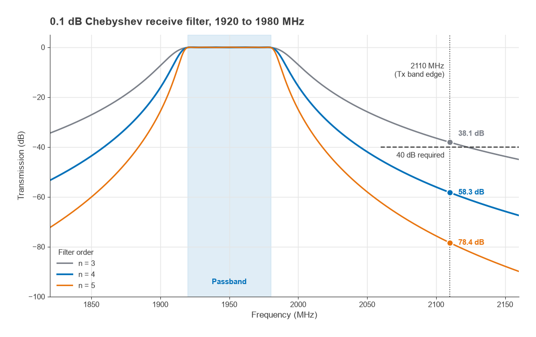
- n = 3: cosh(6.96) ≈ 527, so A ≈ 10 log10(1 + 0.02329 × 5272) ≈ 38.1 dB. Not enough.
- n = 4: A ≈ 58.3 dB. This meets the requirement with margin for manufacturing tolerance and temperature drift.
- n = 5: A ≈ 78.4 dB, at the cost of more loss.
Each added resonator gives roughly 20 dB more rejection at this offset. Real filters often add transmission zeros, placed by cross-coupling non-adjacent resonators, which buy rejection at a particular frequency without adding a full resonator.
Step 3: Estimate Insertion Loss
The 0.1 dB ripple, n = 4 prototype has g1 to g4 = 1.1088, 1.3062, 1.7704 and 0.8181, which sum to 5.0035. With f0/BW = 32.50:
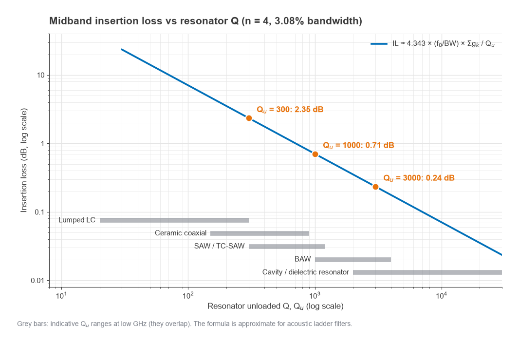
- Qu = 300: IL ≈ 4.343 × 32.50 × 5.0035 / 300 ≈ 2.35 dB
- Qu = 1000: IL ≈ 0.71 dB
- Qu = 3000: IL ≈ 0.24 dB
For a base station receiver this filter sits ahead of the LNA, so its loss adds directly to the system noise figure. The difference between 2.35 dB and 0.24 dB is about 2.1 dB of sensitivity, which in a link budget is worth a significant amount of range. That is why tower-top and base station receive filters use high-Q cavity resonators, while handsets accept acoustic filters with lower Q because of size.
Filter Technologies
Lumped LC
Discrete or integrated inductors and capacitors are cheap and flexible, and they can be made tunable with varactors or switched capacitors. Inductor Q limits them, typically to well under a few hundred for surface-mount parts and lower still on chip. They suit wide fractional bandwidths, harmonic filters after a PA, IF and baseband filters, and anti-aliasing filters. Narrow LC filters at gigahertz frequencies are lossy.
Ceramic (Dielectric) Resonator Filters
Coaxial resonators and monoblock filters use a high-permittivity ceramic to shrink a quarter-wave transmission-line resonator. The physical length scales as 1/√εr. At 1.9 GHz the free-space wavelength is 157.9 mm, so an air quarter-wave resonator is 39.5 mm long; with εr = 90 it shrinks to 39.5 / √90 ≈ 4.2 mm. Q is moderate, in the hundreds, and power handling is better than acoustic filters. Ceramic filters are common in land mobile radio, older handset designs and low-power infrastructure.
SAW
Surface acoustic wave filters launch an acoustic wave along the surface of a piezoelectric substrate, usually lithium tantalate or lithium niobate, using interdigital transducers. Because acoustic velocity is about five orders of magnitude lower than the speed of light, the resonators are tiny. Resonator SAW filters arranged in ladder or lattice configurations dominate handset filtering below about 2.5 GHz. Standard SAW has a large negative TCF; temperature-compensated SAW, which adds a silicon dioxide overlay, reduces it considerably. Above roughly 2.5 GHz the electrode pitch becomes very fine and performance degrades.
BAW
Bulk acoustic wave filters use a thin piezoelectric film, typically aluminum nitride or scandium-doped aluminum nitride, sandwiched between electrodes. The acoustic wave travels through the thickness of the film, and the film thickness sets the frequency. The resonator is acoustically isolated either by an air cavity beneath it (FBAR) or by a Bragg reflector stack (SMR). BAW resonators reach higher Q than SAW at gigahertz frequencies, extend well above 3 GHz, and have lower TCF and better power handling, which makes them the usual choice for demanding handset bands and duplexers with narrow guard bands.
Cavity
Metal cavity filters, usually combline or coaxial resonators machined from aluminum and silver plated, achieve unloaded Q in the thousands. Dielectric resonators mounted in cavities go higher still. They handle hundreds of watts, can be tuned by screws, and support cross-coupled topologies with precisely placed transmission zeros. Their size and cost confine them to base stations, broadcast transmitters and microwave links.
| Technology | Approximate Qu at low GHz | Size | Power handling | Typical role |
|---|---|---|---|---|
| Lumped LC | Tens to low hundreds | Small | Low to moderate | Harmonic, IF, wideband |
| Ceramic coaxial | Hundreds | Medium | Moderate | LMR, low-power infrastructure |
| SAW / TC-SAW | Hundreds to about a thousand | Very small | Low (about 1 W class) | Handset bands below 2.5 GHz |
| BAW (FBAR, SMR) | About one to a few thousand | Very small | Low to moderate | Handset bands to 6 GHz and beyond |
| Cavity, dielectric resonator | Thousands to tens of thousands | Large | High | Base station, broadcast, links |
These ranges are indicative and overlap. Acoustic filters are built as ladders of resonators rather than as classical coupled-resonator networks, so the insertion loss formula above gives an estimate rather than an exact answer for them, but the dependence on Q and fractional bandwidth still holds.
Temperature Drift
TCF is easy to overlook until the guard band is narrow. Suppose a filter at 1950 MHz has a TCF of −40 ppm/°C, a value in the range of uncompensated SAW. Over an operating range of −30 °C to +70 °C, a span of 100 °C, the passband moves by
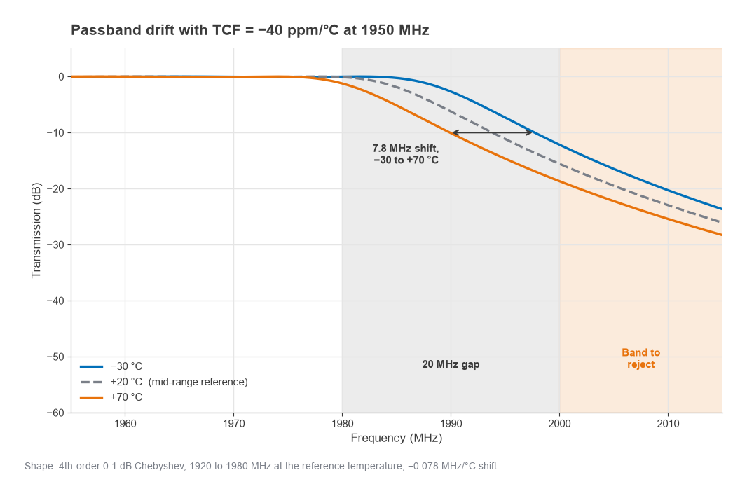
Δf = 40 × 10−6 × 100 × 1950 MHz = 7.8 MHz
If the gap between the passband edge and a band that must be rejected is 20 MHz, nearly 40% of it is consumed by temperature alone, before manufacturing spread is counted. Halving the TCF with a compensated design recovers almost 4 MHz. Self-heating from transmit power at the filter adds to the ambient shift, which is why power handling and TCF are often specified together.
Next in the Series
Filters keep unwanted signals out of the radio, but the local oscillator puts its own impurities directly into the mixer. Part 10, Frequency Synthesis, PLLs and Phase Noise, covers integer-N and fractional-N synthesizers, how phase noise arises and is shaped by the loop, and how to turn a phase noise plot into RMS jitter, EVM and reciprocal mixing.