

The first five parts of this series followed the signal inward, from the antenna through the low-noise amplifier, mixers and filters to the analog-to-digital converter covered in Part 5, ADCs and Receivers. This part reverses the direction. A transmitter starts with bits, turns them into an analog waveform, moves that waveform up to the carrier frequency and raises it to a power level that can cover the required distance. Many of the building blocks are the same ones already discussed for receivers, but the priorities change.
In a receiver the main worries are sensitivity and the ability to survive strong unwanted signals. In a transmitter the worries are spectral purity, modulation accuracy and power efficiency. The transmitter is the only part of the radio that can interfere with other users, so regulators specify what it may emit both inside and outside its own channel. The architecture chosen decides how hard it will be to meet those limits.
What a Transmitter Has to Do
Every transmitter performs four tasks. It generates the baseband modulation, usually as digital in-phase (I) and quadrature (Q) samples. It converts those samples to analog, either at baseband, at an intermediate frequency (IF) or directly at RF. It translates the signal to the carrier frequency with one or more mixers. Finally it amplifies the result in a driver and power amplifier (PA) and filters it before the antenna.
The performance of the chain is judged by a handful of figures:
- Error vector magnitude (EVM), the RMS difference between the transmitted constellation and the ideal one, expressed in percent or dB. It covers in-channel distortion, noise, phase noise and I/Q errors.
- Adjacent channel leakage ratio (ACLR), the power falling into the neighboring channel relative to the wanted channel. PA nonlinearity is usually the main contributor.
- Spurious emissions, discrete tones and wideband noise far from the carrier, including harmonics, LO leakage and mixer products.
- Efficiency, the fraction of DC supply power that ends up as RF power at the antenna. The PA dominates this number.
The noise floor of a transmitter also matters, particularly in frequency-division duplex (FDD) systems. Wideband noise from the transmit chain that lands in the receive band at the same antenna degrades the receiver’s sensitivity directly, which is one reason duplexers need so much isolation. That topic returns in Part 14.
The Superheterodyne Transmitter
The superheterodyne, or two-step, transmitter mirrors the superheterodyne receiver of Part 2. The baseband signal is first modulated onto a fixed IF, filtered there, and then mixed up to the final RF frequency with a tunable LO. Because the IF is fixed, the channel filtering and the I/Q modulation can be done at one frequency where good filters and accurate quadrature generation are easy to achieve.
The cost is the second mixing step. A mixer produces both the sum and the difference of its inputs, so the upconverter creates the wanted signal at fLO + fIF and an unwanted image at fLO − fIF (or the other way round for high-side injection). The LO itself also leaks through the mixer. Both must be removed by a bandpass filter after the mixer, and the difficulty of that filter is set by the frequency plan.
Worked Example: A Superheterodyne Frequency Plan
Consider a transmitter with an output at 2140 MHz and an IF of 200 MHz, using low-side LO injection. The LO must sit at 2140 − 200 = 1940 MHz. The upconverting mixer then produces:
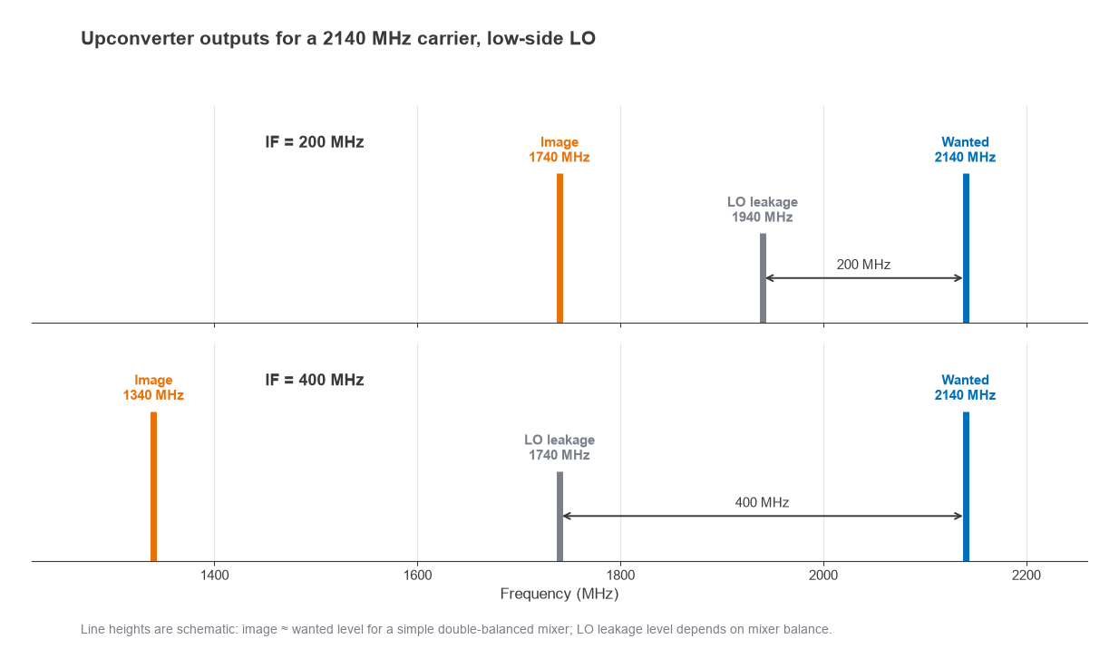
- The wanted signal at 1940 + 200 = 2140 MHz.
- The image at 1940 − 200 = 1740 MHz, at roughly the same level as the wanted signal for a simple double-balanced mixer.
- LO leakage at 1940 MHz, typically 20 to 40 dB below the LO drive level depending on mixer balance.
The nearest unwanted product, the LO, is only 200 MHz away from the carrier, or about 9.3% of the output frequency. A filter that passes the wanted channel and gives, say, 60 dB of rejection 200 MHz away at 2 GHz is achievable, but it needs several resonators and adds loss. Raising the IF to 400 MHz pushes the LO to 1740 MHz and the image to 1340 MHz, which eases the filter. The price is a harder IF stage, since a higher IF makes the IF filter and the I/Q modulator more demanding. This tradeoff, between IF difficulty and RF filter difficulty, is the central design decision in a superheterodyne transmitter.
A sideband-rejecting (image-reject) upconverter, built from two mixers driven in quadrature, can cancel the image before filtering. It relaxes the filter but does not remove the LO leakage, so a post-mixer filter is still needed.
Direct-Conversion (Zero-IF) Transmitters
In a direct-conversion transmitter, analog I and Q baseband signals drive a quadrature modulator clocked by an LO at the carrier frequency. There is no IF, no IF filter and no image in the superheterodyne sense. The architecture needs fewer parts and integrates well on silicon, which is why it is now the usual choice in handsets, Wi-Fi radios and many small-cell and macro base station designs.
Direct conversion brings its own impairments, each tied to the fact that the LO sits in the middle of the wanted channel.
LO Leakage (Carrier Feedthrough)
DC offsets in the baseband path and imperfect mixer balance let some LO energy through to the output. It appears as a tone at the channel center and is visible as an offset of the constellation origin. It cannot be filtered because it is in-band. Calibration loops measure the leakage, often with a feedback receiver, and apply small DC corrections to the I and Q DACs to null it.
I/Q Imbalance and Sideband Suppression
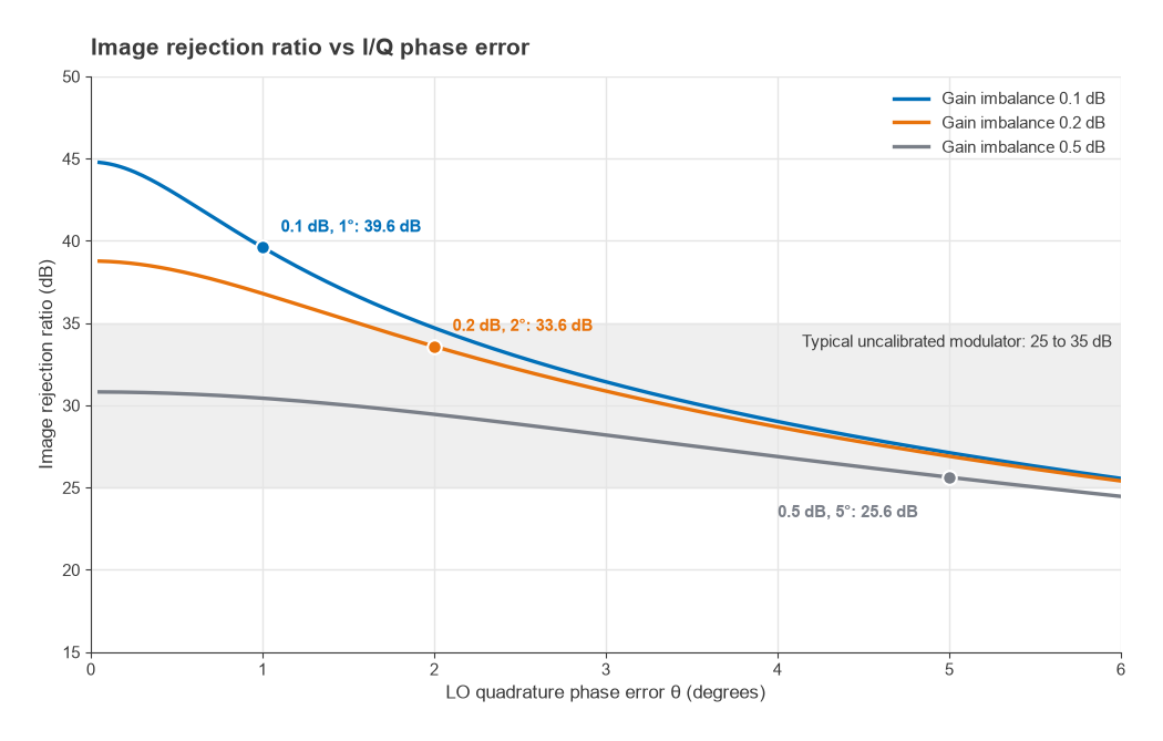
If the I and Q paths do not have identical gain, or the LO phases are not exactly 90° apart, part of the signal appears as a mirror image reflected about the carrier. For a gain mismatch ratio (1 + ε) and a phase error θ, the image rejection ratio is
IRR = 10 log10 [ (1 + 2(1 + ε)cos θ + (1 + ε)2) / (1 − 2(1 + ε)cos θ + (1 + ε)2) ] dB
Take a gain imbalance of 0.2 dB and a phase error of 2°. Then 1 + ε = 100.2/20 = 1.0233 and cos 2° = 0.99939. The numerator is 1 + 2(1.0233)(0.99939) + 1.0471 = 4.0925. The denominator is 1 − 2.0453 + 1.0471 = 0.0018 (more precisely 0.00179). The ratio is about 2286, so IRR ≈ 33.6 dB. Loosening the match to 0.5 dB and 5° drops the IRR to about 25.6 dB, while tightening it to 0.1 dB and 1° raises it to about 39.6 dB. Uncalibrated analog modulators commonly land in the 25 to 35 dB range, and digital pre-correction of gain and phase is used where better figures are required.
LO Pulling
The PA output is a large signal at the same frequency as the VCO in the synthesizer. Coupling through the substrate, supply or package can pull the VCO, modulating its frequency with the transmitted envelope. The common fix is to run the VCO at twice (or another multiple of) the carrier and divide down, or to offset it with a mixer, so that the VCO frequency does not coincide with the strong PA output.
Building an EVM Budget
Because uncorrelated error sources add in power, an EVM budget is assembled as a root-sum-square of the individual contributions. Three are usually large enough to matter: I/Q image, LO phase noise and PA distortion.
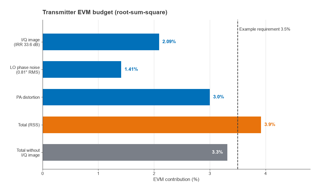
An image at −IRR dBc behaves like an uncorrelated error signal, so its EVM contribution is 10−IRR/20. With the 33.6 dB IRR above, that is 10−33.6/20 ≈ 2.09%.
Phase noise contributes an EVM approximately equal to the RMS phase error in radians. Suppose the synthesizer has an integrated RMS phase error of 0.81°, which is 0.0141 rad. That adds about 1.41%. Part 10 shows how this figure is derived from a phase noise plot.
Assume the PA, operating at its intended back-off with whatever linearization is fitted, contributes 3.0%. The total is
EVMtotal = √(2.092 + 1.412 + 3.02) = √(4.37 + 1.99 + 9.00) = √15.36 ≈ 3.9%
If the standard demands, for example, 3.5% at the antenna, the budget shows where to work. Removing the I/Q contribution entirely would give √(1.99 + 9.00) ≈ 3.3%, so calibrating the modulator to 40 dB IRR or better would likely be enough. Halving the phase noise contribution alone would not. The root-sum-square nature of the budget means the largest term always deserves attention first.
Polar, Outphasing and Envelope-Tracking Transmitters
Cartesian (I/Q) transmitters require a linear PA, and linear PAs are inefficient when driven with signals that have a high peak-to-average power ratio (PAPR). Several architectures attack that problem by splitting the signal into components that are easier to amplify efficiently.
A polar transmitter expresses the signal as an amplitude A(t) and a phase φ(t). The phase drives a constant-envelope path, often a phase-modulated PLL, feeding a saturated, highly efficient PA. The amplitude modulates the PA supply voltage. This is the envelope elimination and restoration (EER) idea first proposed by Kahn. Its weak points are the wide bandwidth of the amplitude and phase signals, which are much wider than the original I/Q signal, and the need to align the two paths in time very accurately. A timing mismatch between amplitude and phase paths shows up directly as spectral regrowth.
Envelope tracking (ET) is a gentler version. The PA remains a linear amplifier, but its supply voltage follows the envelope so that the device always operates close to compression. The supply modulator only has to track the envelope approximately, which relaxes its bandwidth and accuracy compared with EER. ET is widely used in handset PAs.
An outphasing (LINC, linear amplification with nonlinear components) transmitter splits a variable-envelope signal into two constant-envelope signals with a time-varying phase difference. Each drives a saturated PA, and the outputs are summed in a combiner. When the phases align the output is maximum; when they oppose, the output cancels. With an isolating combiner the efficiency falls at low output because the cancelled power is dumped in the combiner’s resistor. Non-isolating Chireix combiners recover much of that loss at the expense of some linearity.
Choosing an Architecture
The table below summarizes the main tradeoffs. None of the entries is absolute; good calibration and careful layout move every architecture’s limits.
| Architecture | Main strengths | Main weaknesses | Typical uses |
|---|---|---|---|
| Superheterodyne | Fixed-IF filtering, good I/Q accuracy, LO away from carrier | More parts, image and LO filtering at RF | Microwave links, legacy base stations, test equipment |
| Direct conversion | Simple, small, easy to integrate, wide tuning | LO leakage, I/Q imbalance, LO pulling | Handsets, Wi-Fi, most modern base stations |
| Polar / EER | Efficient saturated PA | Wide amplitude and phase bandwidth, path alignment | Low-to-moderate bandwidth handset designs |
| Envelope tracking | Improved efficiency with linear PA | Supply modulator design and bandwidth | Handset PAs |
| Outphasing | Saturated PAs, potentially high efficiency | Combiner loss or linearity tradeoff | Research and specialized infrastructure |
| Direct RF DAC | No analog mixer, multiband from one chain | DAC power, spectral purity, clock quality | Wideband and multiband infrastructure |
The last row anticipates Part 11. Modern RF DACs can sample fast enough to synthesize carriers in the low gigahertz range directly, removing the analog upconverter and with it the LO leakage and I/Q imbalance problems. They trade those for the DAC’s own spurious products, images at multiples of the sample rate and the need for a very clean sampling clock.
Whatever architecture is chosen, the last active stage is almost always a power amplifier, and its efficiency and linearity shape the rest of the design. A PA that must stay linear will usually be backed off from its peak capability, and that back-off costs supply power and heat. Understanding where the efficiency goes requires looking at how PAs are biased and loaded.
Next in the Series
Part 7, Power Amplifiers, Classes and Efficiency, looks at the final stage in detail: conduction angle, the theoretical efficiency limits of Class A, B, AB and C, switching amplifiers, and how back-off and signal PAPR determine the efficiency a real transmitter actually achieves.