Linearity and Distortion in RF Circuits

An RF circuit is nonlinear when its output is no longer a scaled copy of its input, so that doubling the input does not double the output and new frequencies appear that were not present at the input. Linearity in RF design is the study of how far a circuit departs from that ideal, which signal levels make the departure visible, and which specifications (P1dB, IP3, IP2, SFDR, blocking) put numbers on it.

Every active device is nonlinear to some degree. Transistor current depends exponentially or quadratically on control voltage, junction and drain capacitances change with voltage, and supply rails and temperature move with the signal. At low levels these effects are small enough to ignore. At the levels found in a crowded band, or at the output of a power amplifier, they set the limit on what a radio can do. This hub introduces the model behind all linearity specifications and links to the pages that treat each one in detail, as part of the wider RF design reference.

The Power-Series Model of a Nonlinear Circuit

For a circuit that is only mildly nonlinear and has no memory, the output y can be written as a Taylor series in the input x:

y(t) = a₁x(t) + a₂x²(t) + a₃x³(t) + …

The coefficient a₁ is the small-signal voltage gain. The a₂ term comes from asymmetry in the transfer curve, and a₃ from its curvature. For a compressive amplifier a₃ has the opposite sign to a₁, which is why gain falls as the drive rises. Higher-order terms exist, but the first three explain almost every specification on an amplifier or mixer datasheet.

Substituting a single tone x = A cos(ωt) gives a fundamental of amplitude a₁A + (3/4)a₃A³, a second harmonic of (1/2)a₂A² and a third harmonic of (1/4)a₃A³. The first expression already contains gain compression: once (3/4)|a₃|A² is no longer small compared with a₁, the fundamental falls below the straight-line extrapolation. Setting that shortfall to 1 dB gives the 1 dB compression point.

Two tones and intermodulation

With two tones of equal amplitude A at f₁ and f₂, the cubic term produces products at 2f₁ − f₂ and 2f₂ − f₁ with amplitude (3/4)|a₃|A³. These third-order intermodulation (IM3) products are the troublesome ones, because they sit right next to the wanted signals where no filter can remove them. In dB terms they grow 3 dB for every 1 dB increase in input, while the fundamental grows 1 dB. Extrapolating the two straight lines until they meet defines the third-order intercept point, IP3. The square term produces second-order products at f₂ − f₁ and f₁ + f₂, which grow 2 dB per dB and define IP2.

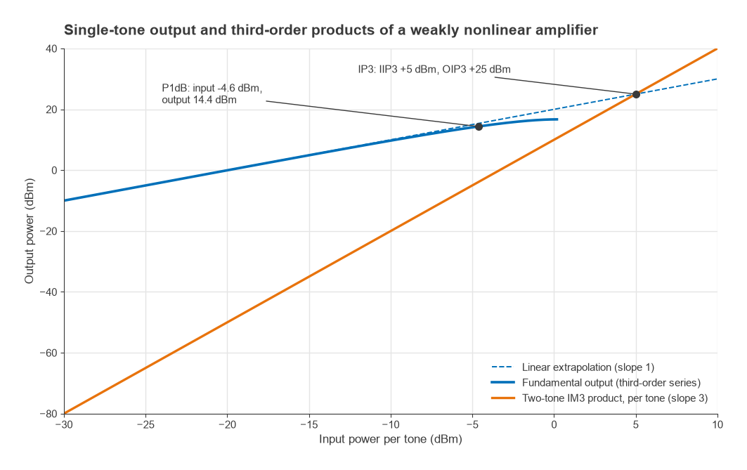
Output power versus input power showing the fundamental, its linear extrapolation, the IM3 line, P1dB and IP3 — Figure 1: Fundamental and IM3 output of an amplifier with 20 dB gain and IIP3 of +5 dBm, computed from a third-order power series. The input P1dB falls about 9.6 dB below IIP3.

Those slopes give the two working equations used throughout this branch. For input power P_in per tone, output power P_out per tone and gain G, all in dB units:

P_IM3,out = 3P_in − 2·IIP3 + G = 3P_out − 2·OIP3
P_IM2,out = 2P_in − IIP2 + G

For a pure third-order nonlinearity the same coefficients fix both the compression point and the intercept point, and the input-referred IP3 lands about 9.6 dB above the input 1 dB compression point. Real devices are close to that relationship but not bound by it, which is why datasheets list both numbers.

A worked example

Take an amplifier with 20 dB gain, IIP3 = +5 dBm and IIP2 = +25 dBm, driven by two tones of −20 dBm each at 100 MHz and 110 MHz. The fundamentals come out at about 0 dBm. The IM3 products at 90 MHz and 120 MHz are 3(−20) − 2(5) + 20 = −50 dBm, 50 dB below each tone. The second-order products at 10 MHz and 210 MHz are 2(−20) − 25 + 20 = −45 dBm. A time-domain simulation of the same power series, transformed with an FFT, returns exactly those levels, along with second harmonics at −51 dBm and third harmonics at about −59.5 dBm.

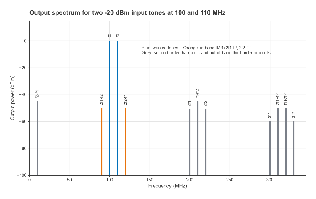
Output spectrum with two tones at 100 and 110 MHz, IM3 products at 90 and 120 MHz, and second and third-order products — Figure 2: FFT of the same amplifier driven by two -20 dBm tones. IM3 products sit at -50 dBm, second-order sum and difference products at -45 dBm.

Raise each input tone by 10 dB, to −10 dBm, and on the straight-line model the IM3 products climb 30 dB to −20 dBm, only 30 dB below tones of about +10 dBm. In practice the amplifier is by then within a few dB of compression, so the real figures are somewhat worse. That threefold growth is why a receiver that behaves well at moderate levels can collapse quickly when a strong neighbour appears.

Where Nonlinearity Shows Up in a Radio

The same handful of coefficients appears under different names depending on the signal environment:

Effect	Main cause	Usual specification	Where it hurts
Gain compression	a₃ opposing a₁	P1dB, Psat	PA output, receiver overload
Third-order intermodulation	a₃	IIP3, OIP3	Adjacent signals in receivers, spectral regrowth in transmitters
Second-order distortion	a₂	IIP2	Zero-IF and wideband receivers
Harmonics	a₂, a₃	dBc at 2f, 3f	Transmitter spurious emissions
Blocking and desensitization	a₃ with one strong tone	Blocking level, desense in dB	Receivers near strong transmitters
AM-AM and AM-PM conversion	Level-dependent gain and phase	Degrees per dB, EVM, ACLR	High-PAPR transmitters

The lower end of the usable signal range is set by noise, covered in the RF noise branch. The upper end is set by the effects in this table. The span between them is the dynamic range, and most front-end trade-offs, from LNA gain to mixer drive level, are attempts to move one boundary without dragging the other along with it.

Pages in This Section

1 dB Compression Point (P1dB) and Gain Compression: definition, measurement, input versus output P1dB, saturation and the link to IP3.
Intermodulation and Intercept Points: Radio Architectures Part 3, deriving IM3, IP3 and IP2 for receivers.
Cascaded IP3 and System Linearity: how the intercept points of several stages combine, and why the last stage usually dominates.
Dynamic Range and SFDR: the span between the noise floor and the level at which distortion becomes visible.
Blocking, Desensitization and Reciprocal Mixing: what a single strong interferer does to a receiver’s sensitivity.
Harmonic Distortion and AM-AM / AM-PM Conversion: harmonics, phase distortion and their effect on modulated signals.

Several existing pages apply these ideas to complete radios. Radio Architectures Part 2 covers mixer spurs, Part 4 covers sensitivity at the noise end of the range, and PA Linearization shows how feedforward, DPD and Doherty designs recover linearity at high power. Amplifier-specific linearity figures are collected in the RF amplifiers hub.

Frequently asked questions

What makes an RF circuit nonlinear?

The active devices inside it. Transistor current is an exponential or square-law function of control voltage, device capacitances vary with voltage, and bias points shift with signal level and temperature. Any of these makes the transfer curve bend, which creates compression, harmonics and intermodulation.

Why are third-order products more important than second-order ones?

Third-order products such as 2f₁ − f₂ fall next to the wanted signals, inside the passband of any filter that passes them. Second-order products land near DC or near twice the signal frequency, where a bandpass filter usually removes them. The exception is the zero-IF receiver, where second-order products fall directly on the baseband signal.

Is a passive circuit always linear?

Mostly, but not completely. Ferrite components, switch diodes, corroded connectors and dissimilar metal contacts can all generate weak intermodulation, known as passive intermodulation (PIM). It matters most in high-power transmit paths that share an antenna with a sensitive receiver.