

Part 16, Modulation, EVM and Peak-to-Average Ratio, showed how the modulation order fixes the SNR a link must deliver. The link budget in Part 15 supplied that SNR from a short list of lines, two of which were antenna gains entered as single numbers in dBi, and one of which was a free-space path loss. Both simplifications hide a good deal of engineering.
This part looks at antennas and propagation from the radio designer’s side rather than the antenna designer’s. The aim is to understand what the numbers on an antenna datasheet mean, what limits them, and how a real path differs from free space, so that the corresponding lines in the budget can be chosen with some confidence.
Antenna Parameters a Radio Designer Uses
An antenna is a transducer between a guided wave on a transmission line and a wave in free space. Reciprocity means its pattern, gain and impedance are the same in transmit and receive, so the same figures serve both ends of the budget.
Directivity D compares the power density in the direction of maximum radiation with the power density an isotropic radiator would produce with the same total radiated power. It is purely a property of the pattern shape. Gain includes the losses in the antenna itself:
G = ηrad D
where ηrad is the radiation efficiency, the fraction of accepted power that is radiated rather than dissipated in conductors and dielectrics. Gain is quoted in dBi, relative to an isotropic radiator, or in dBd, relative to a half-wave dipole. A lossless half-wave dipole has a directivity of 1.64, so 0 dBd = 2.15 dBi. Mixing the two is a common way to gain or lose 2 dB in a budget without noticing.
Datasheets increasingly quote realized gain, which also subtracts the mismatch loss at the antenna terminals. That is the figure a link budget wants, since mismatch loss is real power not radiated. Part 14 covered how VSWR translates into mismatch loss and why handset antennas need tuners as their environment changes.
The rest of a datasheet describes the pattern: the half-power beamwidth in each principal plane, the sidelobe level, the front-to-back ratio, and the cross-polar discrimination. The impedance bandwidth, usually defined by a return loss limit such as 10 dB, tells the designer over what range the gain figures apply.
Aperture, Gain and Beamwidth
For an antenna with a physical aperture, such as a reflector or a horn, gain is tied to area by
G = 4πAe/λ2
where Ae is the effective aperture, the physical area multiplied by an aperture efficiency ηap. A uniformly illuminated aperture has ηap = 1 in principle, but its edge illumination spills energy past the rim, so practical feeds taper the illumination towards the edge. That lowers the efficiency, broadens the main beam and reduces the sidelobes. Efficiencies of 0.55 to 0.7 are typical for reflector antennas. For a circular dish of diameter Dant the gain becomes
G = ηap(πDant/λ)2
Gain and beamwidth are two sides of the same aperture. A uniformly illuminated circular aperture has a half-power beamwidth of about 59λ/Dant degrees and a first sidelobe at −17.6 dB. With a parabolic taper that falls to zero at the rim, the beamwidth widens to about 73λ/Dant and the first sidelobe drops to −24.6 dB. The rule of thumb θ3dB ≈ 70λ/Dant describes the tapered illumination of a typical dish.
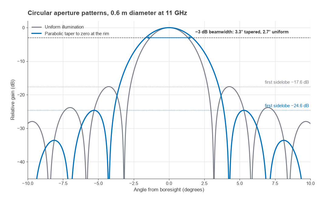
Consider a 0.6 m dish at 11 GHz with ηap = 0.6. The wavelength is λ = 3 × 10⁸/11 × 109 = 27.27 mm, so πDant/λ = 69.1 and
G = 0.6 × 69.12 = 2865, or 34.6 dBi
The beamwidth is about 70 × 0.02727/0.6 = 3.2°. A 3° beam is narrow enough that the mounting matters: a mast that twists by 1.6° in wind moves the far end to the half-power point and costs 3 dB. High-gain links are as much a structural problem as an RF one.
At the other extreme are antennas much smaller than a wavelength, such as those in handsets and IoT modules. The Chu limit sets the minimum radiation Q of an antenna that fits inside a sphere of radius a:
Qmin = 1/(ka)3 + 1/(ka), with k = 2π/λ
Bandwidth falls roughly as 1/Q. At 900 MHz (λ = 333 mm), an antenna confined to a sphere of 40 mm radius has ka = 0.754 and Qmin = 3.66, which allows a fractional bandwidth of at most about 27%. Halving the radius raises Qmin nearly sixfold. Small antennas can be matched over a wider band only by adding loss, which lowers efficiency, which is why the low bands in a handset are always the hardest to cover.
Polarization
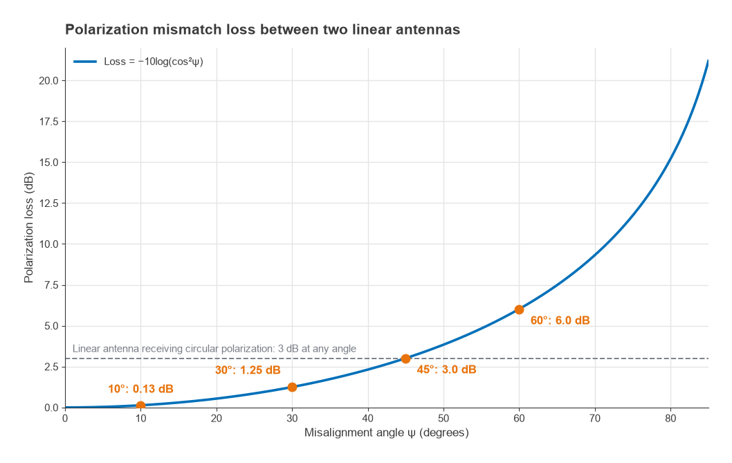
The polarization of an antenna is the orientation of the electric field it radiates. Two linearly polarized antennas whose polarization planes differ by an angle ψ couple with a polarization loss factor
PLF = cos2ψ
A 10° error costs 0.13 dB, 30° costs 1.25 dB, 45° costs 3.0 dB and 60° costs 6.0 dB. At 90° the theoretical loss is infinite, and in practice it is limited by the cross-polar discrimination of the antennas and by depolarization along the path. A linearly polarized antenna receiving a circularly polarized wave loses 3 dB at any orientation, which is why circular polarization is used where the orientation of one end is unknown or rotates, as in satellite links and some RFID systems.
Orthogonal polarizations can also be used deliberately. A dual-polarized antenna with ±45° slant elements gives two nearly independent ports in one housing, which provides polarization diversity, or two spatial streams for the MIMO techniques covered in the next part. For a handset held at an arbitrary angle, a single linear polarization at the base station would lose several dB on average, and dual-polarized receive antennas recover most of that.
Near Field, Far Field and Placement
Gain and pattern are far-field quantities. They describe the antenna at distances where the wavefront is effectively plane and the field falls as 1/r. The usual boundary for an antenna of largest dimension Dant is the Fraunhofer distance
Rff = 2Dant2/λ
For the 0.6 m dish at 11 GHz, Rff = 2 × 0.36/0.02727 = 26.4 m. A gain or pattern measurement made closer than that will be wrong, which is why large antennas are measured on long outdoor ranges, in compact ranges, or with near-field scanners and a transformation. Inside about 0.62√(Dant3/λ), 1.75 m for the same dish, is the reactive near field, where stored energy dominates and nearby objects detune the antenna rather than merely blocking it.
For small antennas the reactive region is a fraction of a wavelength, but in a compact product that fraction contains the battery, the display, the shield cans and the user’s hand. The antenna’s performance in the finished product can differ by several dB from its performance on an evaluation board. Two antennas inside the same enclosure also couple to each other, which reduces isolation between radios and degrades the diversity and MIMO gains that two antennas are meant to provide.
Propagation Beyond Free Space
Free-space loss assumes a single direct path. Over flat ground, the simplest correction adds one reflected ray. With antenna heights ht and hr, the direct and reflected paths differ in length by about 2hthr/d, and at grazing incidence the ground reflection coefficient is close to −1. Close in, the two rays alternately reinforce and cancel. Beyond the breakpoint distance
db = 4hthr/λ
they cancel progressively, and the path loss tends to
PL = 40log(d) − 20log(hthr)
with d and the heights in metres. The loss now rises at 40 dB per decade instead of 20, and it no longer depends on frequency, while raising either antenna by a factor of two gains 6 dB.
Real environments add buildings, foliage and terrain. The most common engineering abstraction is the log-distance model with shadowing:
PL(d) = PL(d0) + 10n log(d/d0) + Xσ
where n is the path loss exponent (2 in free space, commonly around 3 to 4 in built-up outdoor areas) and Xσ is a zero-mean Gaussian variable in dB with standard deviation σ, often in the range of 6 to 10 dB. Shadowing is slow: it changes over tens of metres as the terminal moves behind or out from buildings, unlike the multipath fading of Part 15, which changes over a fraction of a wavelength. A budget that must hold at a given fraction of locations at the cell edge adds a shadowing margin of zpσ, where zp is the Gaussian quantile for that fraction. For 90% of locations, zp = 1.28.
Worked Example: A 900 MHz Mobile Path
A base station antenna at ht = 30 m serves a handset at hr = 1.5 m, 5 km away, at 900 MHz. The wavelength is 0.333 m.
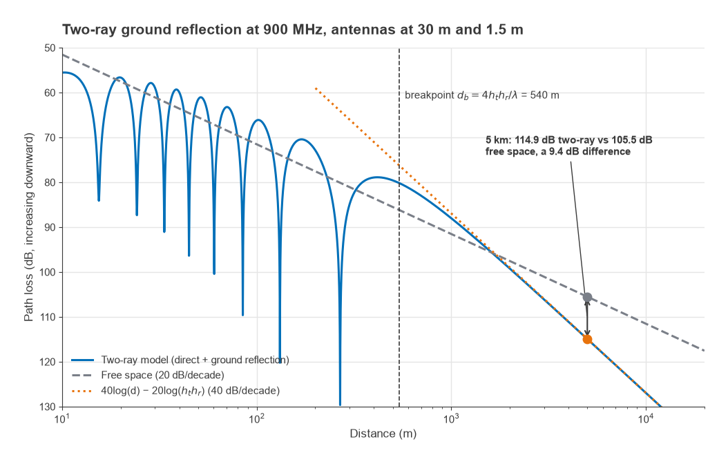
- Free-space loss: 20log(5) + 20log(900) + 32.44 = 13.98 + 59.08 + 32.44 = 105.5 dB.
- Breakpoint: db = 4 × 30 × 1.5/0.333 = 540 m, so 5 km is well beyond it.
- Two-ray loss: 40log(5000) − 20log(45) = 147.96 − 33.06 = 114.9 dB.
- Shadowing margin for 90% of locations with σ = 8 dB: 1.28 × 8 = 10.3 dB.
- Polarization loss for a handset tilted 45° to a single vertically polarized base antenna: 3.0 dB.
The ground reflection alone adds 9.4 dB to the free-space figure, and the location margin and polarization add another 13.3 dB. Together these are 22.7 dB, close to the entire 25 dB margin of the line-of-sight link in Part 15, and that is before any allowance for clutter or for Rayleigh fading. A full exact two-ray calculation at 5 km gives 114.9 dB, matching the asymptotic formula. Near the breakpoint it does not: at 540 m the two rays add in phase and the received level is 6 dB above free space.
The example shows where the useful levers are. Antenna height is worth 6 dB per doubling at the base station. Dual-polarized base station antennas remove most of the polarization loss. Shadowing can only be covered by margin, by denser sites, or by diversity between sites that are not shadowed at the same time. None of these is visible in a budget that uses free-space loss, which is why free space is suitable for line-of-sight links like the one in Part 15 and optimistic almost everywhere else.
Next in the Series
A single antenna has a fixed pattern. Several antennas driven together can steer a beam, null an interferer or carry several data streams at once. Part 18, MIMO, Beamforming and Phased-Array Architectures, covers array gain, beam steering, grating lobes and the analog, digital and hybrid architectures used to build them.