Microstrip Design and Impedance Calculator

A microstrip line is a planar transmission line formed by a conducting strip on one side of a dielectric substrate with a ground plane on the other, and its characteristic impedance depends on the strip width W, the substrate height h and the relative permittivity ε_r. To calculate it, find the effective permittivity ε_eff from W/h and ε_r, then apply the Hammerstad closed-form equations for Z₀. The calculator on this page does both directions: impedance from width, and width from a target impedance.

Microstrip is the default interconnect on RF printed circuit boards because it is easy to fabricate, easy to probe and easy to attach components to. It belongs to the transmission line theory section of the RF design map, alongside the general types of transmission lines and the line parameters that the formulas below summarize.

Microstrip Geometry and the Quasi-TEM Mode

In a coaxial cable or a stripline, the field lives entirely in one dielectric and the wave is pure TEM. Microstrip is different. Most of the electric field runs straight down through the substrate, but part of it fringes through the air above the strip. Because the wave travels partly in air and partly in dielectric, it cannot be pure TEM. At the frequencies where microstrip is normally used, the longitudinal field components are small, and the line behaves as if it were a TEM line filled with a single uniform material of permittivity ε_eff, where 1 < ε_eff < ε_r. This is the quasi-TEM approximation, and every closed-form microstrip formula relies on it.

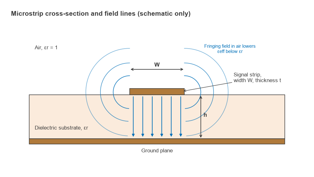
Microstrip cross-section showing strip width W, substrate height h, ground plane and fringing field lines — Figure 1: Microstrip cross-section with field lines (schematic only). Fringing through the air makes the effective permittivity lower than the substrate's.

Once ε_eff is known, the other line properties follow directly. The phase velocity is v_p = c/√ε_eff, the guided wavelength is λ_g = c/(f√ε_eff), and the delay per unit length is √ε_eff/c. Wider strips put more of the field in the substrate, so ε_eff rises toward ε_r and Z₀ falls.

Effective Permittivity

The Hammerstad expressions for the static effective permittivity, with u = W/h, are

For u ≤ 1: ε_eff = (ε_r + 1)/2 + (ε_r − 1)/2 × [ (1 + 12/u)^−1/2 + 0.04(1 − u)² ]
For u ≥ 1: ε_eff = (ε_r + 1)/2 + (ε_r − 1)/2 × (1 + 12/u)^−1/2

The first term, (ε_r + 1)/2, is the average of air and substrate, which is the limit for a very narrow strip. The second term pushes ε_eff toward ε_r as the strip widens.

Hammerstad and Wheeler Closed-Form Equations

With ε_eff in hand, the characteristic impedance for a strip of negligible thickness is

For u ≤ 1: Z₀ = (60/√ε_eff) ln(8/u + u/4)
For u ≥ 1: Z₀ = 120π / [ √ε_eff (u + 1.393 + 0.667 ln(u + 1.444)) ]

For design, the inverse problem is more useful: given Z₀ and ε_r, find W/h. Wheeler’s synthesis equations, in the form given in most microwave textbooks, are

A = (Z₀/60)√((ε_r + 1)/2) + ((ε_r − 1)/(ε_r + 1))(0.23 + 0.11/ε_r)
B = 377π / (2Z₀√ε_r)
For W/h < 2: W/h = 8e^A / (e^2A − 2)
For W/h > 2: W/h = (2/π)[ B − 1 − ln(2B − 1) + ((ε_r − 1)/(2ε_r))(ln(B − 1) + 0.39 − 0.61/ε_r) ]

Accuracy

These simple forms are generally quoted as accurate to roughly 1 percent against full-wave solutions for zero-thickness strips over the usual range of W/h. The fuller Hammerstad and Jensen (1980) model, which includes strip thickness and a more elaborate ε_eff expression, is considerably more accurate and is what most commercial calculators implement. In practice the formula is rarely the largest error. The permittivity of a laminate can vary by several percent from its nominal value and with frequency, and finished copper and dielectric thicknesses carry their own tolerances. A 5 percent error in h moves Z₀ by about 1.5 Ω on a 50 Ω line, far more than the difference between formula versions. Copper thickness t reduces Z₀ slightly; a common correction widens the strip by ΔW = (t/π)(1 + ln(2h/t)), which for 35 µm copper on 1.6 mm FR-4 is about 0.06 mm. For final designs, especially at millimetre-wave frequencies, check the result with an EM field solver.

Characteristic impedance versus W/h for relative permittivity 3.66, 4.3 and 10.2 — Figure 2: Z0 versus W/h from the Hammerstad equations. 50 Ω needs W/h = 1.96 at εr = 4.3 and 2.21 at εr = 3.66.

Worked Example: 50 Ω on 1.6 mm FR-4

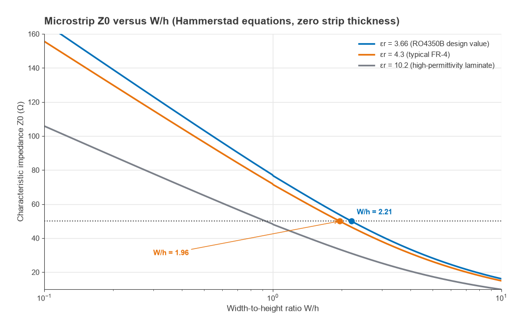
Design a 50 Ω line on a 1.6 mm board with ε_r = 4.3, a typical value for FR-4 near 1 GHz.

Synthesis: A = (50/60)√(5.3/2) + (3.3/5.3)(0.23 + 0.11/4.3) = 1.357 + 0.159 = 1.516. Then W/h = 8e^1.516/(e^3.032 − 2) = 1.945, which is below 2, so the first formula applies. W = 1.945 × 1.6 = 3.11 mm.
Check with the analysis equations: u = 1.945 gives ε_eff = 3.266 and Z₀ = 50.2 Ω. Iterating the analysis equations to exactly 50.0 Ω gives W/h = 1.961, or W = 3.14 mm, with ε_eff = 3.268. The two methods agree within about 1 percent.
Line properties: √ε_eff = 1.808, so the delay is 6.03 ps/mm and the static guided wavelength at 2.4 GHz is 69.1 mm, so a quarter-wave section is about 17.3 mm long. Including dispersion (next section) shortens the wavelength slightly, to about 68.7 mm.
Thickness correction: with 35 µm copper the effective width grows by about 0.06 mm, so the drawn width for 50 Ω falls to roughly 3.08 mm.

A 3 mm trace on 1.6 mm FR-4 analyses to 51.4 Ω, which shows how forgiving the geometry is: a 0.14 mm change in width moves the impedance by only about 1.4 Ω.

50 Ω Width Table for Common Stackups

Because Z₀ depends only on W/h and ε_r, the 50 Ω width scales linearly with substrate height. The table uses zero-thickness strips, ε_r = 4.3 for FR-4 and ε_r = 3.66 for RO4350B, which is approximately the manufacturer’s recommended design value for that laminate. Confirm both the permittivity and the finished thickness with the board fabricator before releasing a layout; the trade-offs between the two materials are covered in FR-4 vs Rogers.

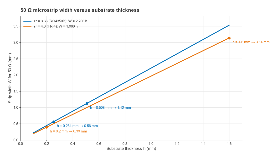
50 ohm strip width versus substrate thickness for FR-4 and RO4350B — Figure 3: The 50 Ω strip width scales linearly with substrate thickness (zero-thickness strips).

Material	ε_r	h (mm)	W for 50 Ω (mm)	ε_eff
FR-4 (thin prepreg layer)	4.3	0.20	0.39	3.27
FR-4	4.3	0.36	0.71	3.27
FR-4	4.3	0.80	1.57	3.27
FR-4	4.3	1.60	3.14	3.27
RO4350B	3.66	0.254	0.56	2.85
RO4350B	3.66	0.508	1.12	2.85
RO4350B	3.66	0.762	1.68	2.85
RO4350B	3.66	1.524	3.36	2.85

The ratio W/h is 1.96 for FR-4 and 2.21 for RO4350B. On a multilayer board where the RF layer sits over a thin prepreg, the 50 Ω trace becomes narrow, which reduces the footprint mismatch at component pads but increases conductor loss. Transmission line losses explains how conductor and dielectric loss scale with width and frequency.

Microstrip Impedance Calculator

Enter the substrate and either a strip width (to analyse) or a target impedance (to synthesize). The calculator uses the Hammerstad equations above with the thickness correction, and estimates dispersion with the Getsinger model described in the next section. Results are first-pass design values, not a substitute for a field solver.

Relative permittivity ε_r Substrate height h (mm) Copper thickness t (µm, 0 to ignore)

Strip width W (mm) Target Z₀ (Ω) Frequency (GHz)

Strip width W	–
Characteristic impedance Z₀	–
Static ε_eff	–
ε_eff at the entered frequency (Getsinger)	–
Guided wavelength λ_g at f	–
Delay	–
Transverse resonance estimate	–

Dispersion and Frequency Limits

The quasi-TEM picture is a low-frequency approximation. As frequency rises, the field concentrates more in the substrate, so ε_eff increases from its static value toward ε_r. This is dispersion, and it lowers the phase velocity and raises the effective impedance seen by a resonator or filter designed with static values. A simple and widely used estimate is Getsinger’s model:

ε_eff(f) = ε_r − (ε_r − ε_eff(0)) / (1 + G(f/f_p)²), with f_p = Z₀/(2μ₀h) and G = 0.6 + 0.009Z₀

For a 50 Ω line on 1.6 mm FR-4, f_p = 12.4 GHz, and ε_eff rises from 3.27 at low frequency to about 3.42 at 5 GHz and 3.69 at 10 GHz. On 0.508 mm RO4350B, f_p is 39 GHz, and ε_eff changes only from 2.85 to 2.91 over the same 10 GHz span. Thin substrates are much less dispersive, which is one reason high-frequency boards use them. More refined models, such as Kirschning and Jansen’s, are used in circuit simulators.

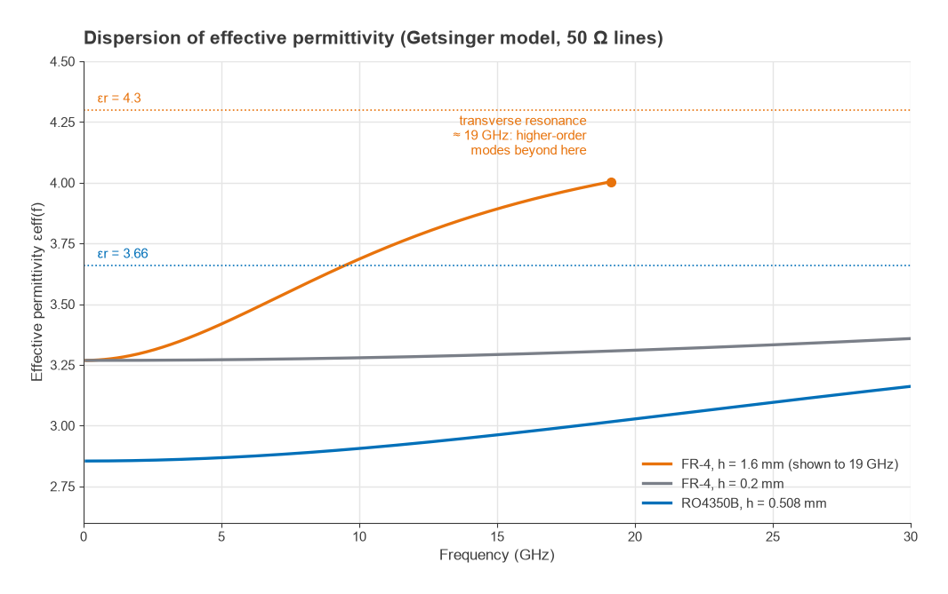
Effective permittivity versus frequency for three 50 ohm microstrip lines using the Getsinger model — Figure 4: Dispersion of εeff for 50 Ω lines (Getsinger model). Thin substrates disperse far less; the 1.6 mm FR-4 curve stops near its transverse resonance.

Two further limits set the useful upper frequency of a given microstrip. A wide strip can support a transverse resonance, a half-wave standing wave across its width, estimated at f_c ≈ c / (√ε_r(2W + 0.8h)). For the 3.14 mm line on 1.6 mm FR-4 this is about 19 GHz. The substrate can also couple strongly to the lowest TM surface wave above roughly f_T = c tan⁻¹(ε_r) / (√2 πh√(ε_r − 1)), which is about 31 GHz for the same board. Designers usually keep the operating frequency well below both, which in practice means choosing a thinner substrate as frequency rises. Radiation from discontinuities and higher losses add further practical limits long before these mode boundaries are reached.

Microstrip vs Grounded Coplanar Waveguide

Grounded coplanar waveguide (GCPW) adds ground copper on the top layer on both sides of the strip, separated by a gap and stitched to the bottom ground with vias. The side grounds pull field out of the substrate and into the gaps, which reduces dispersion, improves isolation between neighbouring lines and gives a shorter ground return for shunt components. The cost is a narrower strip for the same impedance on a given board, more sensitivity to gap tolerance, and the need for a via fence. Microstrip remains simpler and is adequate for most work below a few gigahertz; coplanar waveguide and stripline take over where isolation, dispersion or shielding matter more.

Frequently asked questions

How do you calculate microstrip impedance?

Compute u = W/h, find ε_eff from the Hammerstad expression for the appropriate range of u, then apply the matching Z₀ formula. For design, use Wheeler’s synthesis equations to get W/h from the target impedance and confirm the result with the analysis equations or a field solver.

What trace width is 50 ohm on FR-4?

With ε_r ≈ 4.3, a 50 Ω microstrip needs W ≈ 1.96h. That is about 3.1 mm on a 1.6 mm board and about 0.39 mm over a 0.2 mm dielectric. Because FR-4 permittivity varies between suppliers and with frequency, use the value from the laminate datasheet or the fabricator’s stackup.

Microstrip vs grounded coplanar waveguide?

Microstrip has one strip over a ground plane; GCPW adds top-side grounds and stitching vias next to the strip. GCPW gives lower dispersion and better isolation at higher frequencies, while microstrip is simpler, less sensitive to etch tolerance and adequate for most designs below a few gigahertz.

Does copper thickness change the impedance?

Yes, slightly. Thicker copper behaves like a wider strip and lowers Z₀. For 35 µm copper on 1.6 mm FR-4 the effective width increase is about 0.06 mm, which lowers a 50 Ω line to about 49.4 Ω.