

Part 14, Front-End Modules, Duplexers and Switches, finished the hardware tour at the antenna port. Over fourteen parts this series has built up a transmitter, a power amplifier, filters, synthesizers, converters and several receiver architectures. Each part produced a number or two: a noise figure, an output power, an intercept point, an insertion loss. The link budget is where those numbers meet the path between two antennas and decide whether the radio actually works.
A link budget is an accounting exercise in decibels. It starts with the power leaving the transmitter, adds gains, subtracts losses, and compares what arrives with what the receiver needs. The difference is the margin. The arithmetic is simple, which is precisely why the assumptions behind each line deserve the most care.
The Transmit Side: Power and EIRP
The transmit side of the budget is summarized by effective isotropic radiated power:
EIRP = PTX − LTX + GTX
where PTX is the PA output power in dBm, LTX is the loss in cables, connectors, duplexers and switches between the PA and the antenna, and GTX is the antenna gain in dBi. Regulatory limits are usually written in terms of EIRP or a related quantity, so a higher-gain antenna may require a lower PA output rather than giving more range.
The PTX figure should be the average power the PA can deliver while meeting its linearity requirements, not its saturated output. For a signal with a high peak-to-average ratio, that average sits several dB below saturation, as discussed in Part 7 and Part 8. Using the saturated number is one of the most common ways a link budget ends up optimistic.
The Path: Free-Space Loss and Beyond
In free space, the power received between two isotropic antennas falls with the square of distance. The Friis transmission equation expresses this as a free-space path loss:
FSPL = 20log(4πd/λ)
With d in kilometres and f in megahertz, this becomes the working form
FSPL (dB) = 20log(dkm) + 20log(fMHz) + 32.44
Two features are worth remembering. Doubling the distance adds 6 dB of loss, and so does doubling the frequency. The frequency term is a property of the isotropic antenna’s effective aperture, not of the air: an antenna of fixed physical size gains directivity as frequency rises, which can offset the higher path loss when both ends use fixed-aperture antennas.
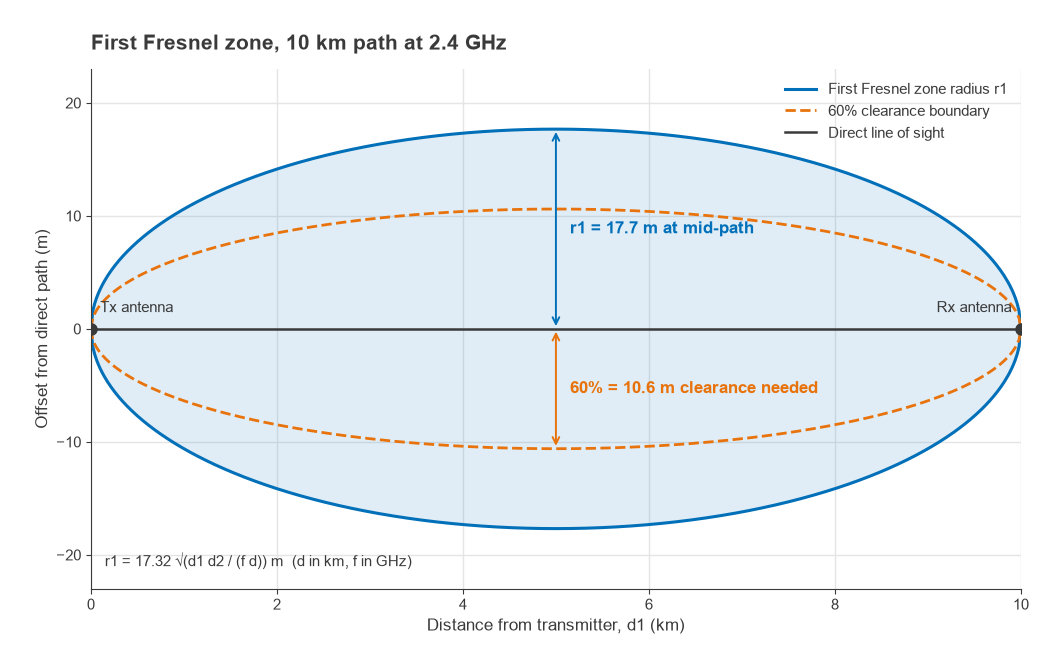
Real paths are rarely free space. Terrestrial links need clearance of the first Fresnel zone, the ellipsoid around the direct path within which reflected signals arrive less than half a wavelength late. Its radius at a point d1 from one end and d2 from the other is
r1 = 17.32 √(d1d2 / (f d)) metres
with distances in kilometres and f in gigahertz. A common design rule is to keep at least 60% of this radius clear of obstructions. Where the path is obstructed or the terminals move through cluttered environments, free-space loss is replaced by empirical models in which loss rises faster than 20 dB per decade of distance, and the model choice can easily shift the result by 20 dB or more. Atmospheric absorption and rain attenuation join the budget at millimetre-wave frequencies.
The Receive Side: Sensitivity
Part 4 derived receiver sensitivity from first principles. The thermal noise power density at 290 K is kT = 1.38 × 10−23 × 290 = 4.0 × 10⁻²¹ W/Hz, which is −174 dBm/Hz. The sensitivity is then
Psens = −174 + 10log(B) + NF + SNRreq
B is the noise bandwidth of the channel in hertz, NF is the cascaded system noise figure, and SNRreq is the signal-to-noise ratio the demodulator needs to meet its target error rate. Each term carries the work of earlier parts. NF comes from the front-end loss and LNA analysis of Parts 4 and 14, and from the converter noise figure in Part 13. SNRreq depends on the modulation and coding, and in practice also on the transmitter’s EVM, the synthesizer’s phase noise (Part 10) and the receiver’s I/Q imbalance (Part 12), since all of those add impairments that behave like extra noise.
Sensitivity alone does not describe a receiver. In a crowded band, the usable sensitivity is often set by blockers through reciprocal mixing, intermodulation and desensitization, which is why the intercept and dynamic range work in Part 3 belongs in any serious system study.
Worked Example: A 10 km Point-to-Point Link
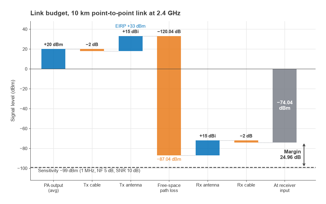
Consider a fixed link at 2.4 GHz over 10 km of clear line-of-sight path. Both ends use identical radios and antennas.
| Item | Value | Running total |
|---|---|---|
| PA output power (linear average) | +20 dBm | +20.0 dBm |
| Transmit cable and connector loss | −2 dB | +18.0 dBm |
| Transmit antenna gain | +15 dBi | +33.0 dBm EIRP |
| Free-space path loss, 10 km at 2400 MHz | −120.04 dB | −87.04 dBm |
| Receive antenna gain | +15 dBi | −72.04 dBm |
| Receive cable and connector loss | −2 dB | −74.04 dBm at receiver input |
The path loss line works out as 20log(10) + 20log(2400) + 32.44 = 20.00 + 67.60 + 32.44 = 120.04 dB.
For the receiver, take a 1 MHz noise bandwidth, a 5 dB noise figure at the receiver input and a demodulator requirement of 10 dB SNR:
Psens = −174 + 60 + 5 + 10 = −99 dBm
The link margin is −74.04 − (−99) = 24.96 dB, about 25 dB. Because the receive cable loss has already been subtracted from the signal, the 5 dB noise figure here must be the receiver’s own figure, not one that includes the cable. Counting the cable in both places is a classic double entry.
The Fresnel zone check at mid-path uses d1 = d2 = 5 km, d = 10 km and f = 2.4 GHz: r1 = 17.32 √(25/24) = 17.32 × 1.021 = 17.7 m. Sixty percent of that is 10.6 m, so the line between the antennas must pass at least 10.6 m above any trees, buildings or terrain near the middle of the path, plus an allowance for earth curvature, which is not negligible at 10 km. If the antennas are mounted too low to achieve that, diffraction loss must be added and the free-space figure no longer applies.
Margin can also be read as range. In free space, every 6 dB of margin doubles the distance, so 24.96 dB corresponds to a factor of 1024.96/20 = 17.7. In principle the same radios would close the link at 177 km. In practice curvature, Fresnel clearance and fading would end that long before, which is the reason margin is not spent on range.
Fade Margin and What the Margin Is For
The 25 dB in the example is not spare. It has to cover everything the budget did not model: multipath fading, antenna misalignment, component ageing, temperature drift in PA output and noise figure, and interference raising the effective noise floor. Of these, fading is usually the largest and the most statistical.
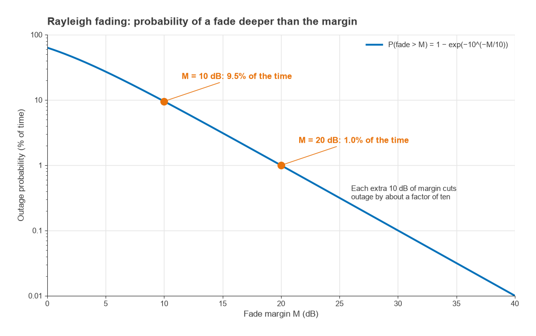
For a mobile link with no dominant path, the received envelope is often modelled as Rayleigh distributed. The probability that the power falls more than M dB below its mean is
P(fade > M) = 1 − exp(−10−M/10)
- M = 10 dB: 1 − exp(−0.1) = 0.095, or 9.5% of the time.
- M = 20 dB: 1 − exp(−0.01) = 0.010, or 1.0% of the time.
Each additional 10 dB of margin reduces the outage probability by roughly a factor of ten in the deep-fade region. This steep cost is the reason diversity, equalization and error-correcting codes exist: they reduce the effective fade depth, so the same availability can be met with less margin. A fixed line-of-sight link with good clearance fades far less than this, but it still needs margin for atmospheric multipath and, at higher frequencies, rain.
When a budget comes up short, the options map directly onto the earlier parts of this series. More PA power or a more efficient, linearized PA (Parts 7 and 8). Lower front-end loss and a better LNA (Parts 4 and 14). Narrower channel bandwidth, which trades data rate for sensitivity at 10log(B). Cleaner synthesizers and converters that lower the SNR the demodulator effectively needs (Parts 10, 11 and 13). Higher-gain antennas, subject to regulatory limits. Every one of them shows up as a line in the table.
Next in the Series
This completes the series. Readers who want to revisit the foundations can return to Part 1, Understand Radio Architectures, where the receiver and transmitter block diagrams used throughout were first introduced. Definitions of the terms used across all fifteen parts are collected in the wireless terms glossary.