

Part 7 showed that a power amplifier is most efficient near saturation and that modern high-PAPR signals force it to operate well below that point. A Class B stage that reaches 70% at peak power drops below 30% at 8 dB back-off. Linearization techniques exist to close that gap, either by making the amplifier behave linearly closer to compression or by changing the amplifier’s operating conditions as the envelope moves.
This part covers the three approaches that have defined infrastructure PA design: feedforward, digital predistortion (DPD) and the Doherty amplifier. The first two correct distortion; the third improves back-off efficiency and relies on the second to clean up the distortion it creates. Most current base station transmitters use some combination of crest factor reduction, DPD and a Doherty or related load-modulated PA.
Describing PA Nonlinearity
Two curves describe a memoryless PA. The AM/AM curve plots output amplitude against input amplitude; it is linear at low drive and flattens into compression. The AM/PM curve plots the output phase shift against input amplitude, which arises from voltage-dependent device capacitances and the changing conduction angle. Both distort a modulated signal, producing in-band error (EVM) and out-of-band spectral regrowth (ACLR).
The third-order intermodulation products discussed in Part 3 are the two-tone view of the same behavior. For a wideband modulated signal, odd-order terms spread the spectrum into the adjacent channels: third-order products occupy up to three times the signal bandwidth and fifth-order up to five times.
Real PAs also have memory. The output depends not only on the present input but on recent inputs, because of bias network impedances at envelope frequencies, thermal time constants and charge trapping in GaN devices. Memory effects show up as asymmetric spectral regrowth and as distortion that changes with signal bandwidth. A linearizer that ignores memory will reach a limit beyond which it cannot improve ACLR further.
Feedforward Linearization
Feedforward is the oldest of the three and works entirely in the analog domain. The input splits into two paths. The main path drives the PA. A sample of the PA output, attenuated by the PA gain, is subtracted from a delayed copy of the clean input; what remains is the distortion alone. That error signal is amplified by a separate, highly linear error amplifier and injected, in antiphase, into the main output through a coupler, with a delay line in the main path to align the two. The distortion cancels and the wanted signal passes.
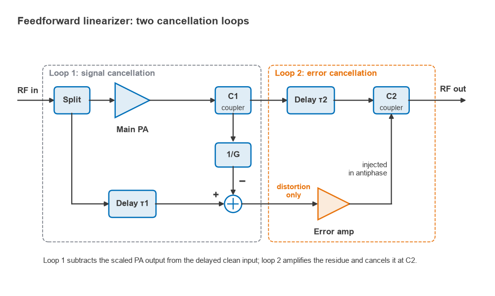
Feedforward handles wide bandwidths and corrects memory effects naturally, since it measures the actual output in real time. Its limitations are the precision of cancellation and the losses it adds.
Worked Example: Cancellation Depth
When two signals of relative amplitude (1 + ε) and relative phase error θ are subtracted, the residual relative to the original is
Cancellation = −10 log10 [ 1 − 2(1 + ε)cos θ + (1 + ε)2 ] dB
For an amplitude mismatch of 0.1 dB, 1 + ε = 100.1/20 = 1.0116. With θ = 1°, cos θ = 0.99985. The bracket evaluates to 1 − 2.02285 + 1.02329 = 0.000443, giving about 33.5 dB of cancellation. With 0.3 dB and 2° the figure falls to about 26.0 dB, and with 0.5 dB and 3° to about 21.9 dB.
Holding 0.1 dB and 1° across a 60 MHz bandwidth, over temperature and aging, is difficult, so practical feedforward systems use adaptive control loops that continuously adjust gain and phase in both the signal-cancellation and error-cancellation loops. Even so, 20 to 30 dB of improvement per loop is a typical practical range.
The losses matter just as much. The delay line and output coupler sit after the main PA, so every decibel of loss there throws away part of the expensive output power. A combined loss of 1 dB means 1 − 10−0.1 = 20.6% of the PA output never reaches the antenna. Add the DC power of the error amplifier, which must itself be very linear, and the overall efficiency of a feedforward amplifier ends up low, often well under 20% for multicarrier designs. This is the main reason DPD displaced feedforward in most new designs.
Digital Predistortion
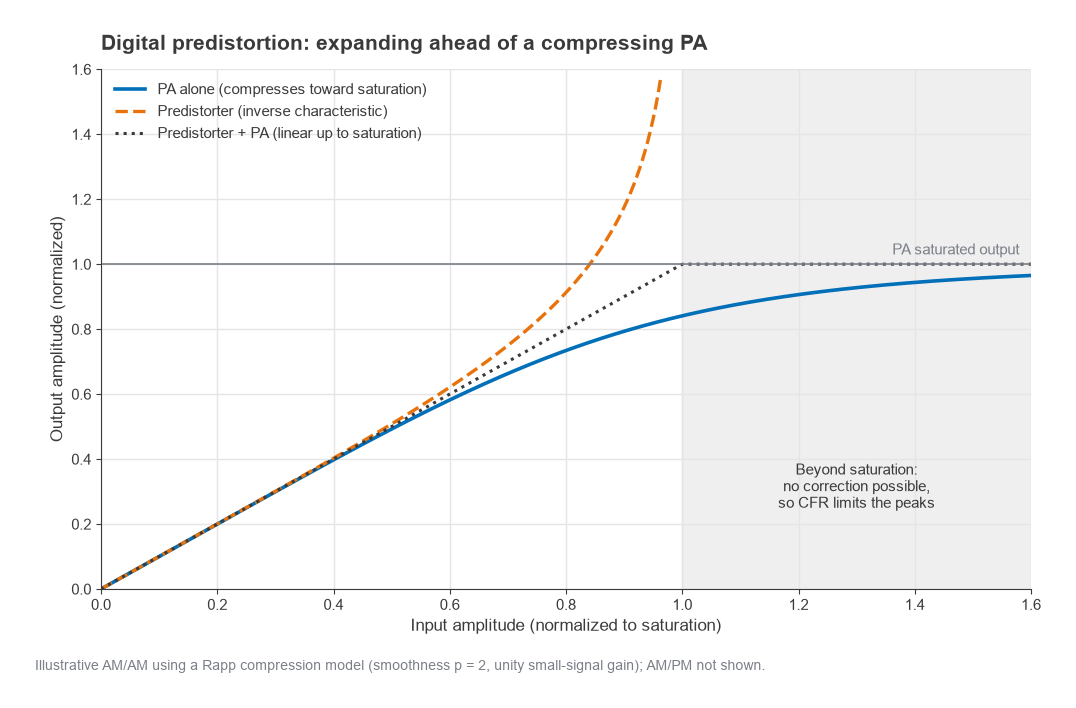
DPD places an inverse nonlinearity in the digital baseband ahead of the DAC. If the PA compresses and rotates phase at high amplitudes, the predistorter expands and counter-rotates by the same amount, so the cascade is linear up to the point where the PA saturates. Nothing can be done beyond saturation: a PA cannot produce more than its maximum output, which is why DPD is always paired with crest factor reduction.
Models
A memoryless polynomial predistorter computes
y(n) = Σk ak x(n) |x(n)|k−1
with only odd k usually needed, since even-order terms fall out of band. To handle memory, the memory polynomial extends this to past samples:
y(n) = Σk Σq akq x(n − q) |x(n − q)|k−1
where q runs over a few memory taps. Generalized memory polynomials add cross terms between the signal and lagging or leading envelope samples. Lookup-table implementations, indexed by input amplitude, are an alternative that maps well to hardware. The coefficients are found by least-squares fitting, using either an indirect learning architecture (fit a post-inverse of the PA, then copy it to the front) or direct learning (adjust the predistorter to minimize the error at the PA output).
The Observation Receiver
DPD needs to see what the PA is actually doing. A coupler at the PA output feeds an observation receiver that downconverts and digitizes the output. Because the predistorted signal contains the inverse distortion products, the DPD output and the observation path must cover several times the signal bandwidth. A common rule is three to five times. For a 20 MHz signal correcting up to fifth order, that is about 100 MHz of observation bandwidth, requiring a complex sample rate of at least 100 MSPS (or a real-sampled ADC above 200 MSPS) and a DAC and transmit path with equally wide passband. For a 200 MHz multicarrier signal, the numbers become challenging, and band-limited DPD variants exist to reduce them.
The observation receiver does not need the sensitivity of the main receiver, but its own linearity and flatness limit what DPD can achieve, since the algorithm corrects whatever it sees, including errors added by the observation path.
The Doherty Amplifier
W. H. Doherty described his amplifier in 1936 for AM broadcast. It returned to prominence in cellular infrastructure because it addresses the back-off efficiency problem directly. A Doherty PA combines a main (carrier) amplifier biased in Class AB or B with a peaking amplifier biased in Class C. Their outputs join through a quarter-wave impedance inverter on the main side.
At low drive the peaking amplifier is off. The impedance inverter presents the main amplifier with twice its optimum load, so it reaches its maximum voltage swing, and therefore peak efficiency, at half its maximum current. For a symmetric design that corresponds to 6 dB below the total peak power. As drive increases beyond that point, the peaking amplifier turns on and injects current into the common node. That raises the apparent impedance at the node, which, through the inverter, lowers the load seen by the main amplifier. The main amplifier stays at full voltage swing while its current, and its output power, keep rising. At full drive both amplifiers see their optimum load and deliver equal power.
Ideal Efficiency Profile
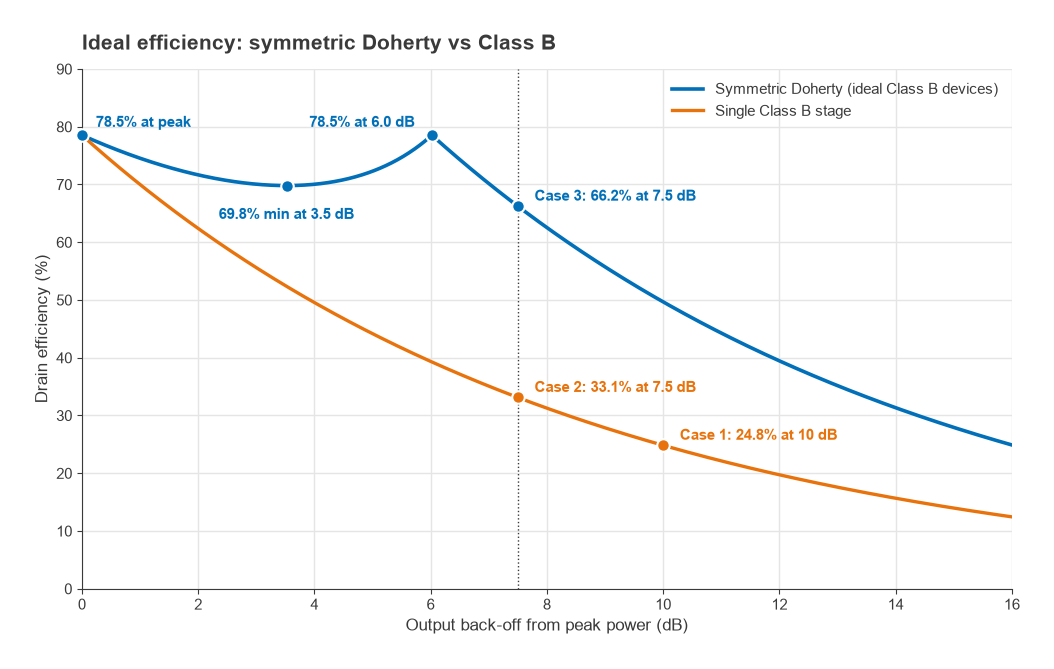
With ideal Class B devices, the symmetric Doherty reaches 78.5% at peak power and again at 6 dB back-off. Between the two peaks, with x defined as the normalized output voltage (0.5 ≤ x ≤ 1),
η = (π/4) · 2x2 / (3x − 1)
Setting the derivative to zero gives a minimum at x = 2/3, which is 3.5 dB below peak, where η = (π/4)(8/9)/1 = 69.8%. Below 6 dB back-off only the main amplifier operates, and efficiency falls as in ordinary Class B: η = (π/4)(x/0.5).
Signals with PAPR above 6 dB benefit from an asymmetric Doherty, in which the peaking device is larger. The back-off point of the first efficiency peak is 20 log10(1 + Ipeak/Imain), with the ratio taken at full drive. Equal currents give 6.0 dB; a peaking amplifier delivering twice the main amplifier’s current gives 20 log10 3 = 9.5 dB. Three-way and multistage Doherty designs extend the high-efficiency region further.
The Doherty is not linear by itself. The peaking amplifier’s Class C turn-on is gradual and nonlinear, and the main amplifier’s load changes with drive, so AM/AM and AM/PM distortion are worse than in a single Class AB stage. The quarter-wave inverter also limits bandwidth, with conventional designs typically covering a fractional bandwidth on the order of 10% to 20%. DPD is therefore part of the design from the start.
Worked Example: What Linearization Buys
Consider a transmitter required to deliver 20 W average. To keep the comparison clean, use ideal Class B efficiency figures; real devices fall short, but the ratios hold.
Case 1, no linearization. Suppose the PA must sit 10 dB below its peak to meet ACLR. Efficiency is (π/4) × 10−10/20 = 0.785 × 0.316 = 24.8%. DC power is 20 / 0.248 = 80.5 W.
Case 2, CFR plus DPD on a Class B PA. CFR reduces the PAPR to 7.5 dB and DPD lets the PA operate just below saturation on the peaks. Efficiency becomes 0.785 × 10−7.5/20 = 0.785 × 0.422 = 33.1%. DC power is 20 / 0.331 = 60.4 W, a saving of 20 W.
Case 3, CFR plus DPD on a symmetric Doherty. At 7.5 dB back-off the Doherty is just below its 6 dB efficiency peak, operating on the main amplifier alone with x = 0.422. Efficiency is (π/4)(0.422/0.5) = 66.2%. DC power is 20 / 0.662 = 30.2 W.
| Configuration | Back-off from peak | Ideal efficiency | DC power for 20 W out |
|---|---|---|---|
| Class B, no linearization | 10 dB | 24.8% | 80.5 W |
| Class B, CFR + DPD | 7.5 dB | 33.1% | 60.4 W |
| Symmetric Doherty, CFR + DPD | 7.5 dB | 66.2% | 30.2 W |
The ideal figures overstate what hardware achieves, because knee voltage, matching loss, imperfect load modulation and the averaging over a real amplitude distribution all reduce efficiency. The ranking, however, holds up in practice: DPD gains through reduced back-off, and the Doherty multiplies that gain by keeping efficiency high where the signal spends most of its time.
Next in the Series
Linearization reduces the PA’s out-of-band emissions, but it cannot remove harmonics, broadband noise or the energy that must be kept out of the co-located receiver. That job falls to filters. Part 9, RF Filters (LC, Ceramic, SAW, BAW, Cavity), compares the filter technologies used across a radio, how resonator Q sets insertion loss, and how to estimate the order a filter needs.