

Part 19, Millimeter-Wave Radio Architectures, ended with arrays whose performance depends on beam direction and which often have no RF connector at all. That is an extreme case of a general problem. Every number in this series, from the noise figure in Part 4 to the link margin in Part 15, is a prediction until someone measures it, and the measurement has errors of its own.
This last part covers four measurements that between them describe most of a radio’s RF performance: noise figure, error vector magnitude, adjacent channel leakage ratio and receiver sensitivity. The emphasis is on what the instrument contributes to the answer, and how to tell when a result describes the test setup rather than the device.
Reference Planes, Calibration and Instrument Limits
Every RF measurement is made at a reference plane, the point at which the instrument’s reading is taken to apply. Cables, adapters, attenuators and fixtures between the instrument and the device all sit between the plane where the instrument is calibrated and the plane the specification refers to. Their loss must be measured and removed, and their mismatch adds uncertainty that a simple loss correction cannot remove. Moving the calibration plane as close to the device as practical is usually the most effective improvement available.
Every instrument also has a floor: displayed noise and distortion in a spectrum analyzer, residual EVM in a vector signal analyzer, the analyzer’s own noise figure, a generator’s level accuracy and leakage. A useful working rule is that the instrument’s contribution to a quantity should sit at least 10 dB below the value being measured. When both contributions are noise-like and add in power, a 10 dB gap still raises the reading by 10log(1.1) = 0.41 dB. A 20 dB gap reduces that to 0.04 dB. Where the gap is smaller, the instrument contribution has to be measured and subtracted, and the uncertainty of that subtraction grows as the gap closes.
Noise Figure: the Y-Factor Method
The most widely used noise figure measurement is the Y-factor method. A calibrated noise source is connected to the input of the device. When the source is off, it presents a noise temperature close to the 290 K reference. When it is on, it presents a higher noise temperature, specified by its excess noise ratio:
ENR = (Thot − 290) / 290
usually quoted in dB. The analyzer measures the output noise power with the source on and off. Their ratio is the Y factor, Y = Non/Noff. With the cold temperature equal to 290 K, the noise factor of everything after the source is
Fsys = ENR / (Y − 1)
with ENR and Y both as linear ratios. This is the noise factor of the device and the analyzer in cascade. The analyzer’s own contribution is removed with the Friis formula from Part 4, which needs the device gain G1 and the analyzer noise factor F2:
FDUT = Fsys − (F2 − 1) / G1
Noise figure analyzers do this automatically, calibrating F2 with the source connected directly and then measuring G1 with the device inserted.
Worked example: an LNA with 20 dB gain
A noise source with ENR = 15 dB (31.62 linear) drives an LNA. The measured Y factor is 11.5 dB (14.13 linear). The LNA gain is 20 dB (100) and the analyzer noise figure is 10 dB (F2 = 10).
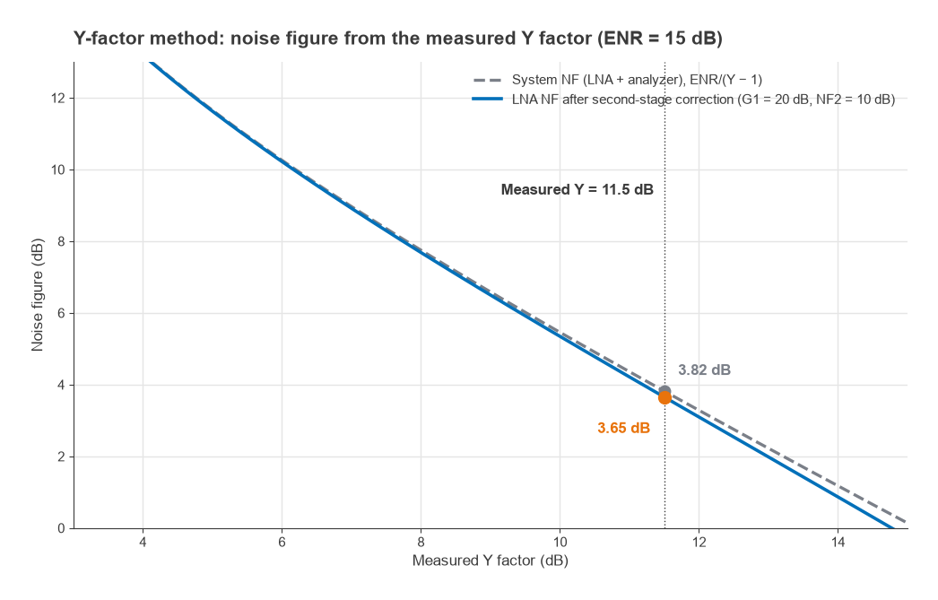
- System noise factor: Fsys = 31.62 / (14.13 − 1) = 31.62 / 13.13 = 2.409, or 3.82 dB.
- Second-stage correction: (10 − 1) / 100 = 0.090.
- LNA noise factor: 2.409 − 0.090 = 2.319, or 3.65 dB.
Ignoring the correction would overstate the LNA noise figure by 0.17 dB here. With a lower-gain device the error grows quickly: at 10 dB gain the correction becomes 0.9, larger than the excess noise of a good LNA. The general guidance follows from the formula. Use a low-noise analyzer, or an external preamplifier ahead of it, when the device gain is low. Choose an ENR that gives a Y factor well above 1, since Fsys is computed from Y − 1 and a small difference between two noisy readings is hard to measure precisely.
Two further error sources are worth knowing. The noise source’s output match changes slightly between its on and off states, which alters the device’s gain and noise behaviour between the two readings. And the formula assumes the cold source is at 290 K. A source at a different physical temperature needs a correction. An alternative, the cold-source or gain method, measures the output noise density directly with the input terminated and computes NF = Nout + 174 − G, with Nout in dBm/Hz and G in dB. It needs an accurately known gain and an analyzer with a very low noise floor, but no noise source.
EVM: Separating the Device from the Analyzer
Part 16 defined error vector magnitude as the rms error vector between the measured symbols and their ideal positions, normalized to the average power of the reference constellation, and noted that some older standards normalize to the peak constellation point instead. Measuring it requires a vector signal analyzer that demodulates the signal, synchronizes timing, frequency and phase, usually equalizes the channel, and then compares each symbol with its ideal position. EVM measured with equalization enabled will hide linear distortion that the same signal shows without it, so the analyzer settings must match the ones the specification assumes.
The analyzer adds its own error vector through phase noise, ADC noise, front-end nonlinearity and I/Q imbalance. The total is called its residual EVM. Because the instrument errors and the device errors are uncorrelated, they add as powers:
EVMmeas2 = EVMDUT2 + EVMinst2
Worked example: correcting for residual EVM
A transmitter measures 2.5% rms EVM on an analyzer whose residual EVM for the same signal and settings is 1.0%. The transmitter’s own EVM is
EVMDUT = √(2.52 − 1.02) = √5.25 = 2.29%
In dB, using 20log(EVM), the measured value is −32.04 dB and the corrected value is −32.80 dB. When the error is dominated by noise-like impairments, EVMrms ≈ 1/√SNR, so the transmitter behaves as if it added noise 32.8 dB below the signal. The correction is meaningful here because the residual is 8 dB below the reading. If the analyzer residual were 2.0%, the corrected answer would depend heavily on how accurately that residual is known, and a better analyzer would be the right fix.
EVM should be measured across the output power range, not only at rated power. At low power it is limited by noise and LO leakage. At high power it rises as the PA compresses.
ACLR and Spectrum Analyzer Dynamic Range
Adjacent channel leakage ratio compares the power a transmitter places in a neighbouring channel with the power in its own channel. Both are measured by integrating the spectrum over the specified channel bandwidth, sometimes with a defined filter shape, and the result is quoted in dBc. A spectrum analyzer measuring ACLR contributes two errors: its own noise integrated across the adjacent channel, and its own intermodulation distortion generated by the strong main-channel signal at its input mixer.
The two behave in opposite ways as the signal level at the mixer changes. Relative to the carrier, the analyzer noise falls 1 dB for each dB of extra signal. Its third-order distortion, relative to the carrier, rises 2 dB for each dB of extra signal, as shown for intercept points in Part 3. There is an optimum mixer level where the two are equal, which is what input attenuator selection is trying to find.
Worked example: finding the analyzer’s ACLR floor
Assume an analyzer with a displayed average noise level of −150 dBm/Hz and a third-order intercept of +15 dBm, both referred to the input mixer, measuring a signal with an 18 MHz channel bandwidth. The analyzer’s own distortion is estimated with the two-tone relation, relative IM3 = 2(P − IP3). With a real modulated signal the figure differs by a few dB, so the result is a guide to setup rather than a guaranteed limit.
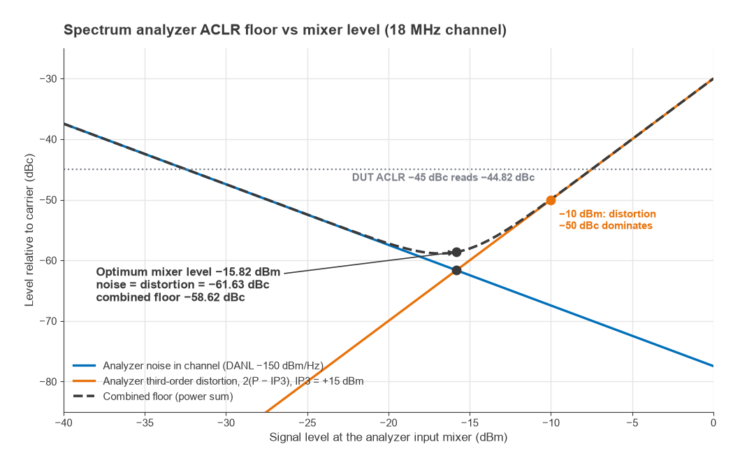
- Noise in 18 MHz: −150 + 10log(18 × 106) = −150 + 72.55 = −77.45 dBm.
- At −10 dBm mixer level: noise is −67.45 dBc, distortion is 2(−10 − 15) = −50 dBc. Distortion dominates.
- Setting −77.45 − P = 2(P − 15) gives P = −15.82 dBm. Both contributions are then −61.63 dBc, and their power sum is −58.62 dBc.
If the transmitter’s true ACLR is −45 dBc and the analyzer contributes −58.62 dBc in power, the reading is 10log(10−4.5 + 10−5.862) = −44.82 dBc, an error of 0.18 dB. Measuring a device with ACLR near −60 dBc would need a better analyzer, noise correction, or a notch filter ahead of the analyzer to remove the main channel. In practice distortion products from the analyzer and from the device can add partly coherently, so the power-sum figure is a typical rather than a worst-case error.
Receiver Sensitivity and Over-the-Air Testing
Conducted sensitivity is measured by connecting a signal generator, through calibrated attenuation, to the receiver’s antenna port and lowering the level until the bit error rate, packet error rate or throughput reaches the threshold the standard defines. The generator is rarely accurate or leak-free at −100 dBm on its own, so it is normally run at a comfortable level and followed by a fixed attenuator. The receiver and the attenuated cable should be inside a shielded enclosure, otherwise radiated leakage from the generator can reach the receiver directly and make it appear more sensitive than it is.
Worked example: checking a sensitivity measurement against prediction
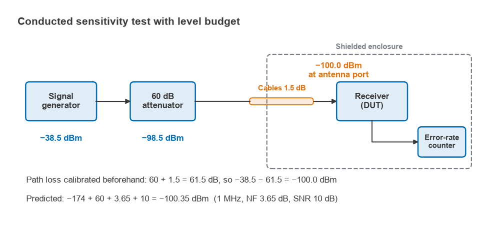
Suppose the LNA measured above sets a receiver noise figure of 3.65 dB, and the receiver needs 10 dB SNR in a 1 MHz noise bandwidth. The predicted sensitivity is
Psens = −174 + 60 + 3.65 + 10 = −100.35 dBm
The test path is a 60 dB fixed attenuator and cables totalling 1.5 dB, both measured beforehand, for 61.5 dB in all. The receiver reaches its error-rate threshold with the generator at −38.5 dBm, which places −38.5 − 61.5 = −100.0 dBm at the antenna port. The result is 0.35 dB worse than predicted, which is within the combined uncertainty of the generator level and the path calibration. A gap of several dB would point to something the budget missed, such as uncounted front-end loss, a demodulator needing more SNR than assumed, or clock harmonics landing in the channel.
Sensitivity in the presence of other signals tells more about a real receiver than sensitivity alone. Adjacent channel selectivity, blocking and intermodulation tests add one or two interfering generators, combined with the wanted signal, and measure how much the wanted signal must be raised to restore the error-rate threshold. They exercise the filters of Part 9, the synthesizer phase noise of Part 10 and the linearity of Part 3 together, which is why they are often the first place a design shows its weaknesses.
When the device has no RF connector, as with the millimetre-wave arrays of Part 19, every one of these measurements moves over the air. EIRP replaces conducted output power, total radiated power integrates it over all directions, and effective isotropic sensitivity replaces conducted sensitivity. The device is measured in an anechoic chamber, often with a compact antenna test range that creates a plane wave in a shorter distance than the true far field. The far-field distance 2D2/λ explains why: for the 42.8 mm square panel of Part 19, the largest dimension D is the 60.5 mm diagonal, and at 28 GHz the far-field distance is 2 × 0.06052 / 0.01071 = 0.68 m. That is manageable for one panel, but it grows with the square of the aperture, and if the whole device radiates, D is set by the device rather than by the panel. Over-the-air uncertainty is generally larger than for the equivalent conducted measurement.
The End of the Series
This completes the Radio Architectures series. Readers can return to Part 1, Understand Radio Architectures, where the block diagrams used throughout were introduced. Definitions of the terms used across the series are collected in the wireless terms glossary.