


RF circuit design is the work of choosing and laying out components so that a high-frequency signal is amplified, filtered or routed with known gain, noise and match. The basics are easiest to learn on one real circuit, so this walk-through designs the input of a 2.4 GHz low noise amplifier (LNA) stage with computed values at every step.
The stage is deliberately small: one transistor, one matching network and its bias. It still contains most of the decisions found in larger RF receiver circuit design. For a map of the whole field, see the RF design guide.
What Is an RF Circuit?
An RF circuit is any circuit where the signal frequency is high enough that parasitics, wavelength and reflections affect the result. At audio frequencies a wire is a wire and a capacitor is a capacitor. At 2.4 GHz a 25 mm trace is a transmission line, and a pad adds capacitance that shows up in the measurement.
Three habits follow from this, and they separate RF electronics design from ordinary circuit design:
- Impedances are complex numbers, and circuits are designed to a reference, usually 50 Ω.
- Results are given as power, gain and noise, not as voltages.
- The layout is part of the circuit. Trace inductance and pad capacitance belong in the calculation.
The RF fundamentals hub and the RF engineering fundamentals article cover the background used here.
RF Circuit Design Example: an LNA Input Stage
An LNA is the first active stage in most receivers, so its noise largely sets the noise of the whole chain. The target for this stage:
- Frequency 2.4 GHz, source impedance 50 Ω
- Input match better than 10 dB return loss across 2.4 to 2.5 GHz
- A mixer stage with 9 dB noise figure follows
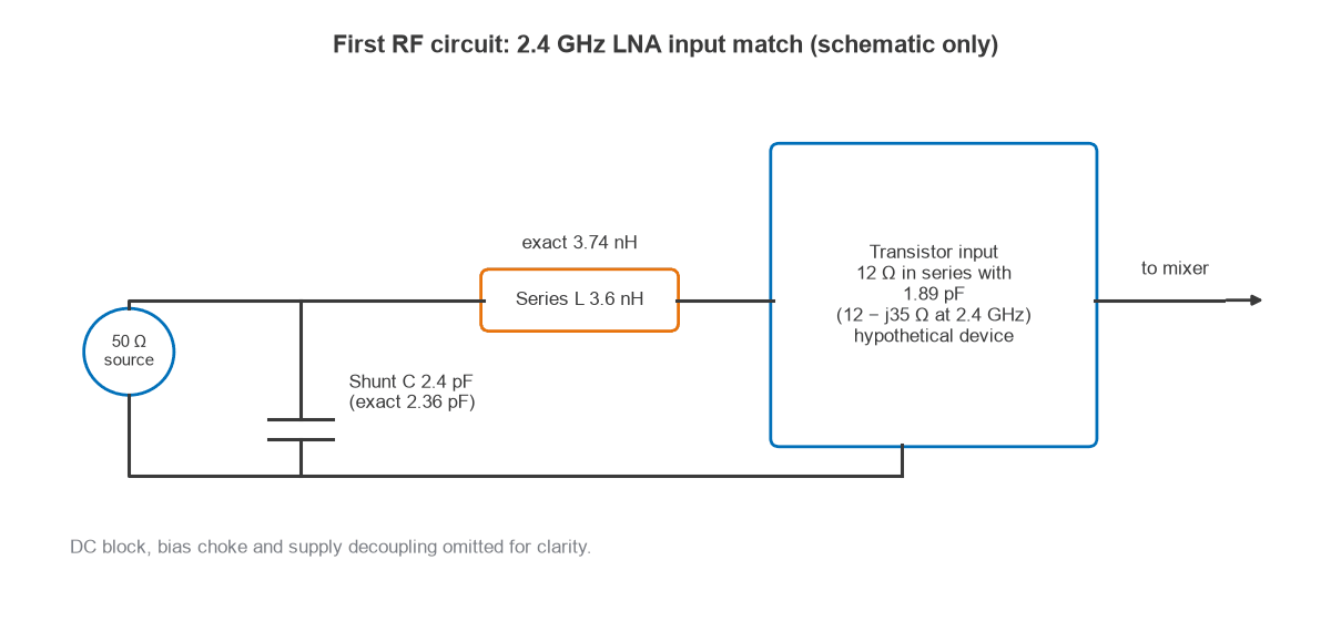
The transistor here is hypothetical, with round numbers standing in for datasheet values: an input impedance of 12 − j35 Ω at 2.4 GHz, modelled as 12 Ω in series with 1.89 pF, plus 16 dB of gain and a 0.8 dB noise figure at the chosen bias. With a real part, these would come from its S-parameter file. See the S-parameters page for how to read one.
Step 1: Compute the Matching Network
Connected directly to 50 Ω, the input would reflect much of the signal. An L-network fixes that with two low-loss parts. The rule is to put the series element next to the lower resistance and the shunt element next to the higher one.
The working, with RL = 12 Ω and RS = 50 Ω:
- Network Q = √(50/12 − 1) = 1.78
- Series reactance for the transformation = Q × 12 = +21.35 Ω
- Series reactance to cancel the input = +35 Ω, giving +56.35 Ω in total
- Inductor L = 56.35 / (2π × 2.4 GHz) = 3.74 nH
- Shunt reactance = 50 / Q = 28.10 Ω
- Capacitor C = 1 / (2π × 2.4 GHz × 28.10) = 2.36 pF
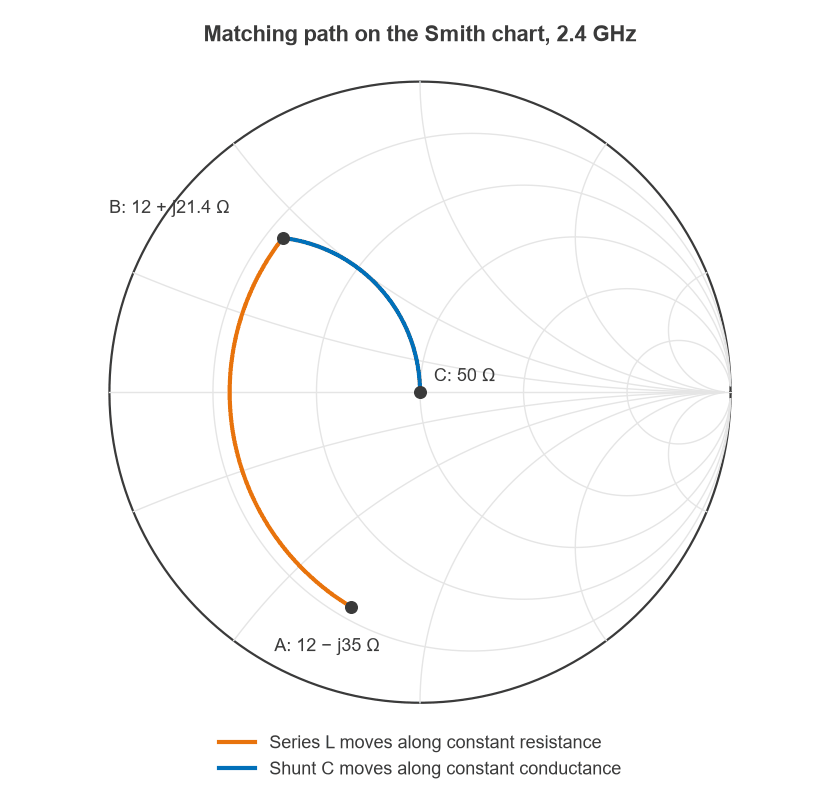
Substituting those values back gives exactly 50 Ω at 2.4 GHz. The Smith chart in Figure 2 shows the same steps as a path. The series inductor moves the impedance from point A to point B, then the shunt capacitor moves it to the centre of the chart at C. The impedance matching calculator will confirm these values, and the Smith chart article explains how to read the path.
Step 2: Use Real Component Values
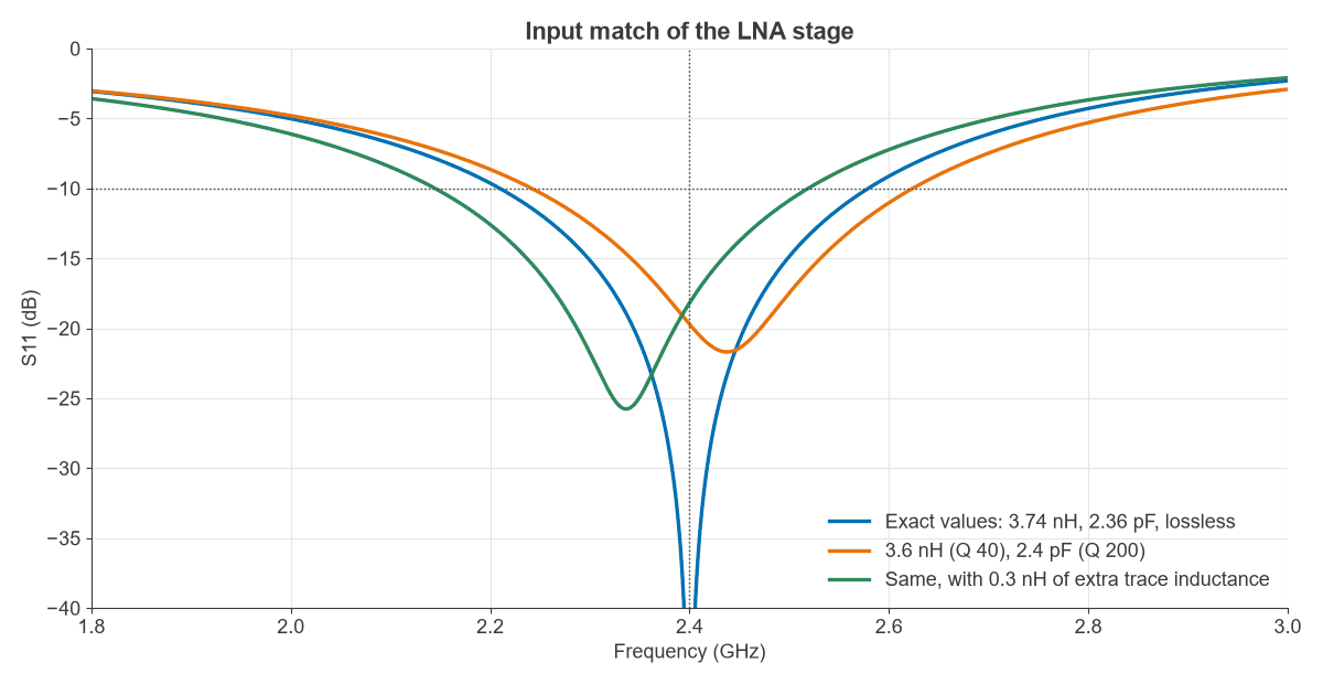
Parts do not come in 3.74 nH. The nearest standard values are 3.6 nH and 2.4 pF, and real parts have loss. Taking an inductor Q of 40 and a capacitor Q of 200, the RF circuit analysis gives:
| Network | S11 at 2.4 GHz | Dip frequency |
|---|---|---|
| Exact, lossless | Perfect match | 2.400 GHz |
| 3.6 nH, 2.4 pF, lossless | −21.9 dB | 2.443 GHz |
| 3.6 nH, 2.4 pF, with loss | −19.7 dB | 2.438 GHz |
| With 0.2 pF of pad capacitance | −17.3 dB | 2.410 GHz |
| With 0.3 nH of trace inductance | −18.2 dB | 2.337 GHz |
With loss, the 10 dB band runs from 2.242 to 2.624 GHz, which comfortably covers the 2.4 to 2.5 GHz target. Figure 3 shows that a few tenths of a nanohenry of trace moves the dip by about 100 MHz, and that is why the layout has to be considered with the circuit. The extra trace case still clears −10 dB at 2.4 GHz and reaches 2.519 GHz at the top edge, so this low-Q match is tolerant. Higher Q matches are not.
Step 3: Check Noise and Gain
Loss in front of the transistor adds directly to noise. The inductor has a reactance of 54.3 Ω, so a Q of 40 means 1.36 Ω of series resistance, in series with the 12 Ω input. Solving the network gives a matching loss of 0.50 dB.
The Friis formula then gives the noise figure of the input loss, transistor and mixer, in linear terms:
F = 1.121 + 0.227 + 0.196 = 1.544, which is 1.89 dB
The three terms are the matching loss, the transistor and the mixer. Without the matching loss, the same chain would be 1.39 dB, so the matching network costs 0.50 dB, nearly all of it in the inductor. Stage gain is 16 − 0.50 = 15.5 dB. In a 1 MHz bandwidth with a 10 dB SNR requirement, the sensitivity at this point would be −174 + 60 + 1.89 + 10 = −102.1 dBm.
One simplification should be stated. This design matches for power. A transistor’s lowest noise comes at a particular source impedance that often differs from the power match, so a real design balances the two. The trade-off is covered in design of radio LNAs.
Step 4: Bias the Transistor
The stage also needs DC, without disturbing the RF path. Take a supply of 3 V and a collector current of 10 mA, with 2 V at the collector, a current gain of 100 and a base-emitter drop of 0.75 V, using collector-feedback bias:
- Collector resistor = (3 − 2) V / 10 mA = 100 Ω
- Base current = 10 mA / 100 = 100 µA
- Feedback resistor = (2 − 0.75) V / 100 µA = 12.5 kΩ
- Power = 3 V × 10 mA = 30 mW
- Transconductance = IC / 25.85 mV = 0.387 S
An RF choke keeps the signal out of the bias network. A 22 nH part is about 332 Ω at 2.4 GHz, large compared with 50 Ω. A 22 pF DC block is about 3.0 Ω, small but not zero, so it should either be included in the match or chosen to run close to its series resonance. More options are on the RF amplifier biasing page.
Step 5: Check Stability and Layout
Gain at one frequency says nothing about whether a stage is stable elsewhere. Any amplifier should be checked for stability using the K factor across the full range where the device has gain, not only in-band. A small series resistor at the output or a resistor in the bias path are common fixes.
Then comes the layout. Keep the input trace short, use a solid ground plane directly under the RF path, place vias next to every ground pad and put decoupling close to the device. Coplanar waveguide and the RF PCB layout page give details. Finish by simulating the whole stage, with free tools or RF simulation software, and measure S11 on a VNA. On a first build, retuning one or two parts is normal.
From One Stage to RF Circuits and Systems
The same five steps apply to most RF components: compute, substitute real parts, check noise or loss, handle DC and check layout. An RF mixer, power amplifier or LC filter changes the priorities, not the method. Integrated RF IC design uses on-chip inductors with lower Q, but the same matching maths. To see how the stages join into a complete receiver, read the radio architectures series.
Frequently Asked Questions
What is an RF circuit used for?
RF circuits generate, amplify, filter, mix and detect high-frequency signals. They are found in radios, phones, Wi-Fi equipment, radar and test instruments, usually between the antenna and the digital part of the system.
What is the difference between RF design and analog design?
RF design treats reflections and power transfer as primary concerns, and works with S-parameters in a fixed impedance system. Low-frequency analog design mostly works with voltages and high-impedance nodes, and can often ignore wavelength.
What are the main components in an RF circuit?
Typical parts are amplifiers, filters, mixers, oscillators, matching networks, switches and transmission lines. Each is specified by gain or loss, noise, linearity and match.
How do I start learning RF circuit design?
Reproduce a calculation like this one, then simulate it, then build it on a small board. The RF engineer roadmap sets out exercises in order.
Related Topics
Continue with RF amplifiers, the RF design guide and the RF calculators. Noise topics are grouped under RF noise.