

RF design is the analysis, synthesis, construction and measurement of circuits and systems that operate at radio frequencies, roughly 3 kHz to 300 GHz, where wavelengths become comparable to the size of the hardware and distributed effects dominate. An RF designer works in terms of power, impedance, noise and distortion rather than node voltages alone, and checks every decision against a specification that is usually written in decibels.
This guide is the entry point to the RF design material on this site. It defines the discipline, walks through the design flow from a requirements sheet to a measured board, introduces the figures of merit that appear in every datasheet and link budget, works one receiver example through by hand, and then maps every section of the site so a reader can go straight to the topic that matters.
What Is RF Design?
RF design covers everything between the antenna and the data converter in a radio, plus the oscillators, synthesizers and power supplies that make that chain work. Its subject matter is the same as analog electronics in principle: amplifiers, filters, mixers and oscillators. What changes is the frequency, and frequency changes the rules.
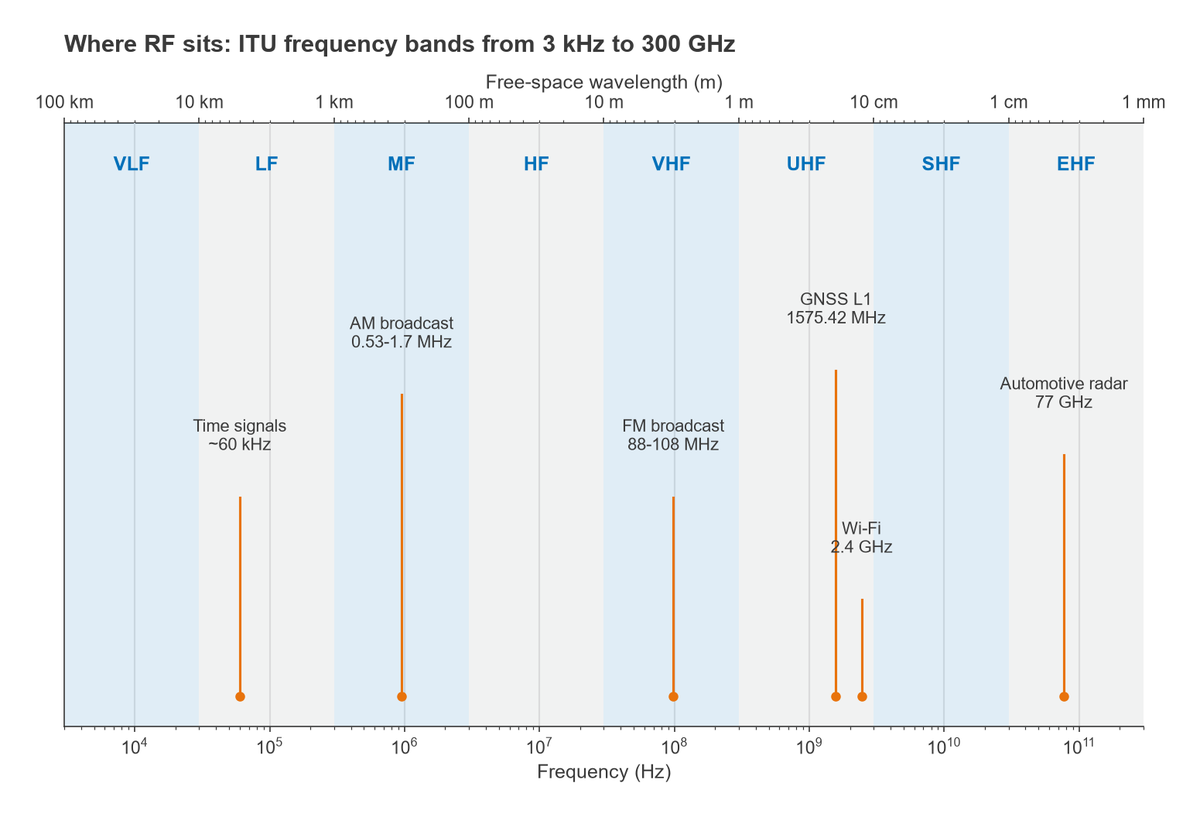
The radio spectrum is conventionally divided into decade bands by the ITU, from VLF (3 to 30 kHz) through LF, MF, HF, VHF, UHF and SHF up to EHF (30 to 300 GHz). The free-space wavelength follows directly from frequency:
λ = c / f
At 3 kHz the wavelength is 100 km. At 1 GHz it is 30 cm, and at 300 GHz it is 1 mm. Inside a circuit board the wave travels more slowly, by a factor of √εeff, so the guided wavelength is shorter still. On a 50 Ω microstrip line over FR-4, where εeff is typically around 3.3, the guided wavelength at 1 GHz is about 16.5 cm. A detailed treatment is in frequency and wavelength in RF design.
Why distributed effects change the method
Low-frequency circuit theory assumes that a wire has the same voltage along its whole length and that a capacitor is only a capacitor. Both assumptions hold while the circuit is much smaller than a wavelength. A common working threshold is one tenth of a wavelength: beyond about λ/10 the phase shift along a conductor reaches 36° and the conductor has to be treated as a transmission line, with a characteristic impedance, reflections and standing waves. Component parasitics follow the same pattern. A 100 pF capacitor with 0.5 nH of package inductance resonates near 712 MHz and looks inductive above that. These effects are why RF engineers think in terms of matched impedances, S-parameters and the Smith chart, and they are the subject of the RF fundamentals section.
What an RF design engineer does
The job varies with the product, but the core tasks are stable. An RF engineer turns a system requirement (range, data rate, channel, regulatory mask, battery life) into a block diagram and a level plan, selects or designs the blocks, matches them to each other, lays out the board or chip so that the layout does not undo the design, and proves the result on the bench with a network analyzer, spectrum analyzer and noise figure meter. Much of the work is bookkeeping in decibels: gain, loss, noise and distortion summed stage by stage until the numbers close.
Who This Guide Is For
The material is written for two readers. Working engineers, including digital, analog, firmware and test engineers who have inherited a radio, can use the section map below as a reference and jump to the calculation they need. Students in electrical engineering courses can read the fundamentals, transmission line, S-parameter, noise and linearity sections in order, then follow the Radio Architectures series, which assembles those ideas into complete receivers and transmitters. Every topic page uses real formulas and at least one worked numeric example, so the reader can check the arithmetic rather than take the result on trust.
The RF Design Flow
Most RF projects follow the same sequence, even if the names and tools differ between companies. The sequence is not strictly linear. Measurement results feed back into component design, and a link budget that will not close forces a return to the architecture or even to the requirements.
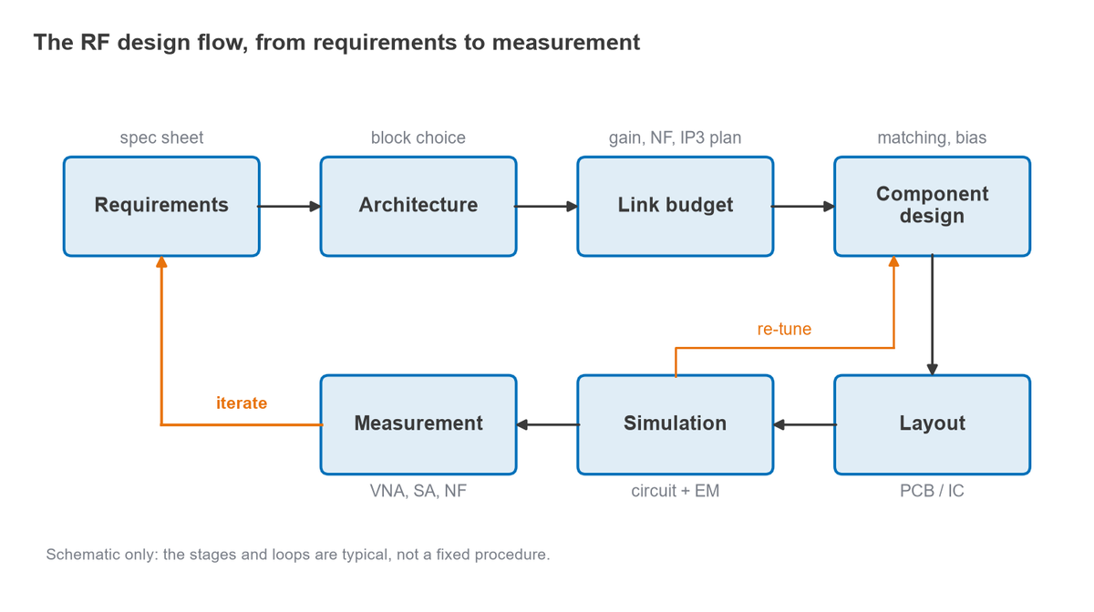
- Requirements. Frequency range, channel bandwidth, modulation, sensitivity, output power, spurious emission limits, power consumption, size and cost. Requirements are written as numbers with units and test conditions.
- Architecture. The choice between superheterodyne, zero-IF, low-IF and direct-sampling receivers, and between direct-conversion and heterodyne transmitters. This choice sets which impairments dominate later.
- Link budget and level plan. The path from transmitter to receiver, then a stage-by-stage table of gain, noise figure and intercept point for each chain. This is where sensitivity and dynamic range are predicted.
- Component design. Matching networks, bias circuits, filters, oscillators and mixers, designed or selected to meet the numbers in the level plan.
- Layout. Controlled-impedance lines, grounding, via stitching, shielding and decoupling. At RF the layout is part of the circuit.
- Simulation. Linear S-parameter simulation, harmonic balance for nonlinear behaviour, and electromagnetic simulation of the layout itself.
- Measurement. S-parameters on a vector network analyzer, spectrum and spurs on a spectrum analyzer, noise figure, phase noise and modulation quality, compared against the original requirements.
The architecture stage is covered by the Radio Architectures series, including Part 15 on link budgets. Layout is covered in RF PCB layout guidelines, and the bench work in RF measurement and test.
Core Figures of Merit
Six quantities appear on nearly every RF datasheet and in every level plan. Each has its own page on this site; the short definitions below are enough to read the rest of this guide.
Gain
Power gain is the ratio of output power to input power, expressed in decibels as G = 10 log10(Pout/Pin). Because RF stages are characterised in a 50 Ω system, the gain on a datasheet is usually the transducer gain |S21|2 measured between 50 Ω terminations. Loss is negative gain, and a passive filter or cable with 2 dB of loss has a gain of −2 dB. Units such as dB, dBm and dBc are explained in dB, dBm, dBW and dBc explained.
Noise figure
Noise factor F is the ratio of input SNR to output SNR when the source is at the reference temperature of 290 K. Noise figure is NF = 10 log10(F). For a cascade of stages, the Friis formula gives the total:
Ftotal = F1 + (F2 − 1)/G1 + (F3 − 1)/(G1G2) + …
with all gains and noise factors as linear ratios. The first stage dominates, which is why a receiver starts with a low noise amplifier. The noise in RF systems section develops this in full.
Linearity: P1dB and IP3
Every amplifier eventually compresses. The output 1 dB compression point (OP1dB) is the output power at which gain has fallen 1 dB below its small-signal value. Two-tone testing produces third-order intermodulation products at 2f1 − f2 and 2f2 − f1, which grow 3 dB for each 1 dB increase in input. Extrapolating the fundamental and the IM3 lines to their crossing gives the third-order intercept point, quoted at the output (OIP3) or input (IIP3 = OIP3 − G). For many amplifiers OIP3 lands roughly 10 dB above OP1dB, but this is a rule of thumb, not a law. The linearity and distortion section covers the derivations.
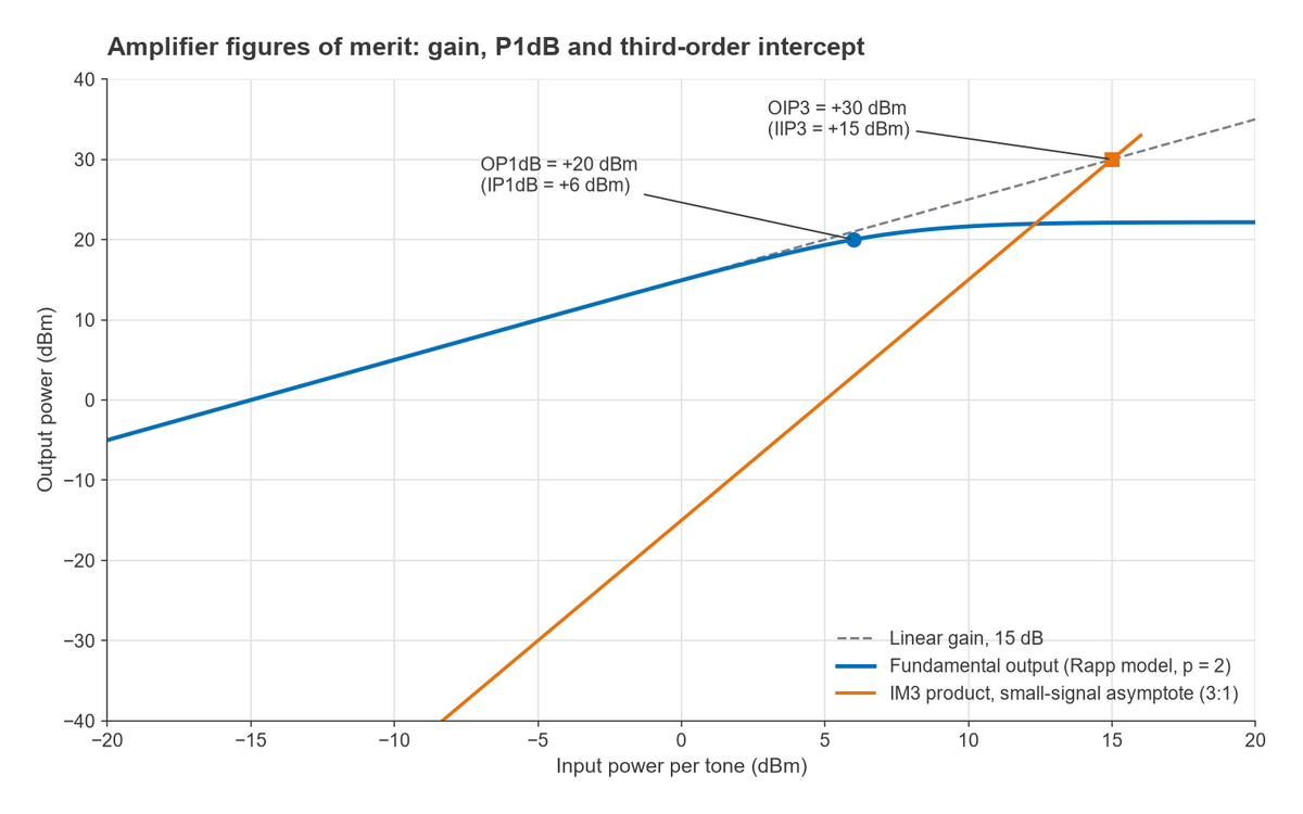
A useful consequence of the 3:1 slope is that the IM3 level for a given tone power can be predicted from the intercept. With output power Pout per tone, the IM3 products sit 2(OIP3 − Pout) dB below the tones. For the amplifier in the figure, at Pout = 0 dBm per tone, they are 2 × (30 − 0) = 60 dB down, at −60 dBm.
Match: return loss and VSWR
The reflection coefficient Γ = (ZL − Z0)/(ZL + Z0) measures how well a load matches the reference impedance. Return loss is RL = −20 log10|Γ| and VSWR = (1 + |Γ|)/(1 − |Γ|). A 75 Ω load on a 50 Ω line gives |Γ| = 0.2, a return loss of 14.0 dB and a VSWR of 1.5. Matching is the subject of the transmission lines and impedance matching section, and the reflection terms S11 and S22 are explained in S-parameters explained.
Efficiency
For power amplifiers, drain efficiency is η = Pout/PDC, and power-added efficiency is PAE = (Pout − Pin)/PDC. A PA delivering 2 W from 5 W of DC power with 0.1 W of drive has η = 40% and PAE = 38%. Efficiency fixes battery life and heat, and it usually trades directly against linearity.
Phase noise
A real oscillator spreads its power into sidebands around the carrier. Phase noise is quoted as single-sideband noise power in a 1 Hz bandwidth at a given offset, relative to the carrier, in dBc/Hz. It limits how close a receiver can operate to a strong neighbour (reciprocal mixing) and how clean a transmitted constellation can be. It is covered in the oscillators and frequency synthesis section.
Worked Example: Receiver Noise Figure and Sensitivity
The following lineup is typical of a simple heterodyne receiver front end. Each stage is described by its gain and noise figure.
| Stage | Gain (dB) | NF (dB) | Friis term | Cumulative NF (dB) |
|---|---|---|---|---|
| LNA | 18 | 1.2 | 1.3183 | 1.20 |
| Band-pass filter | −2 | 2.0 | 0.0093 | 1.23 |
| Mixer | −7 | 8.0 | 0.1334 | 1.65 |
| IF amplifier | 20 | 4.0 | 0.1903 | 2.18 |
The Friis terms are computed with linear values. The LNA contributes F1 = 100.12 = 1.3183. The filter contributes (1.5849 − 1)/63.096 = 0.0093. The mixer sees the LNA gain less the filter loss, a linear gain of 39.81, so it contributes (6.3096 − 1)/39.81 = 0.1334. The IF amplifier sees 63.096 × 0.631 × 0.1995 = 7.94, so its term is (2.5119 − 1)/7.94 = 0.1903. The total is F = 1.6512, or NF = 2.18 dB.
Sensitivity follows from the thermal noise floor of −174 dBm/Hz at 290 K, the noise bandwidth B and the SNR that the demodulator needs:
Pmin = −174 + 10 log10(B) + NF + SNRmin
With B = 1 MHz (60 dB) and a required SNR of 10 dB, Pmin = −174 + 60 + 2.18 + 10 = −101.8 dBm. If the LNA is removed and the chain starts at the filter, the same arithmetic gives a cascaded NF of 13.4 dB and a sensitivity of about −90.6 dBm, more than 11 dB worse. That single comparison explains why front-end design starts with the first gain stage. Part 4 of the series, receiver sensitivity, extends the example.
How RF Design Differs from Analog and Digital Design
Digital design asks whether a signal crosses a logic threshold at the right time. Low-frequency analog design asks how accurately a voltage is reproduced. RF design asks how much power arrives where it should, how much noise and distortion came with it, and how much leaked somewhere it should not. Three practical differences follow.
- Impedance is a design variable. Stages are matched to a reference impedance, usually 50 Ω, so that power transfers cleanly and filters and cables behave as specified.
- Layout is part of the schematic. Trace widths, ground returns and via placement set impedances and coupling, so the same schematic can work or fail depending on the board.
- Specifications are statistical and spectral. Results are expressed as noise densities, spur levels in dBc and masks over frequency, rather than as single voltages.
The boundaries are blurring. Modern radios digitise closer to the antenna, as described in Part 13 on direct RF sampling, and RF integrated circuits mix all three disciplines on one die. The basic RF questions of match, noise and linearity remain.
Map of This Guide
The sections below follow the order in which most courses teach the subject. Each link leads to a section hub that introduces the area and lists its detailed pages.
Foundations
- RF Fundamentals: Units, Waves and Power: decibels, wavelength, power, Q factor, skin effect and component parasitics.
- Transmission Lines and Impedance Matching: characteristic impedance, reflections, VSWR, microstrip, the Smith chart and matching networks.
- S-Parameters Explained: the scattering matrix, gain definitions, stability and Touchstone files.
- Noise in RF Systems: kTB, noise figure, the Friis formula, noise temperature, sensitivity and phase noise.
- Linearity and Distortion in RF Circuits: P1dB, IP3, cascaded linearity, dynamic range and blocking.
Building blocks
- RF Amplifiers: Types, Specs and Selection: LNAs, gain blocks, power amplifiers, biasing and transistor technologies.
- RF Filters: filter specifications, LC and microstrip filters, SAW and BAW, duplexers.
- Oscillators and Frequency Synthesis: PLLs, VCOs, crystal references and direct digital synthesis.
- Mixers and Frequency Conversion: mixer types, image rejection, I/Q modulators and frequency planning.
- RF Passive Components and Building Blocks: couplers, dividers, hybrids, attenuators, circulators, switches, detectors and connectors.
- Antennas and Propagation for RF Designers: antenna parameters, PCB and patch antennas, matching and path loss.
Systems
- Radio Architectures: The Complete 20-Part Series: receivers, transmitters, converters, front ends and link budgets, one block at a time.
- Modulation for RF Designers: analog and digital modulation, OFDM, ACLR and constellation diagrams.
- MIMO Fundamentals: spatial multiplexing, diversity, beamforming and phased arrays.
- RF Design by Application: SDR, GNSS, radar, 5G, satellite and LoRa front ends.
- RFIC Design: An Introduction: integrated RF circuits and how they compare with MMIC and discrete designs.
Practice, tools and learning
- RF PCB Layout Guidelines: stackups, grounding, shielding, decoupling, EMC and coexistence.
- RF Measurement and Test: VNAs, calibration, spectrum analyzers, noise figure and phase noise measurement.
- RF Design Tools, Simulators and Calculators: circuit and EM simulators, free tools and calculators.
- Learning RF Design and RF Engineering Careers: a learning roadmap, books, interview questions and the RF and wireless glossary.
Readers who want a gentler first pass can also start with RF circuit design basics and the Smith chart guide.
Frequently Asked Questions
What frequency range counts as RF?
The usual definition spans about 3 kHz to 300 GHz, which matches the ITU bands from VLF to EHF. The part above roughly 1 GHz is often called microwave, and the part above 30 GHz millimetre-wave. In practice the label matters less than whether the circuit is large compared with a tenth of a wavelength.
What does an RF design engineer do day to day?
An RF engineer writes level plans and link budgets, designs or selects amplifiers, filters, mixers and oscillators, designs matching networks, reviews layouts, runs simulations and measures prototypes. A large share of the time goes into debugging: finding why a measured noise figure, spur or match differs from the prediction.
How is RF design different from analog design?
The circuits are related, but at RF the conductors and components are no longer small compared with a wavelength. Impedance matching, transmission line behaviour, parasitics and layout become first-order effects, and performance is specified in power, noise density and spectral terms rather than voltage accuracy.
What is the RF design flow from spec to measurement?
A typical flow runs requirements, architecture, link budget and level plan, component design, layout, simulation and measurement. Results from simulation and measurement loop back to component design or to the architecture until the measured performance meets the specification.
Related Topics
Good next steps from here are dB and dBm for the units used throughout, S-parameters for how RF blocks are described, noise and linearity for the two limits on dynamic range, and the Radio Architectures series for complete systems. The older overview article on radio frequency design remains available as a shorter introduction.