

The 1 dB compression point (P1dB) is the signal level at which an amplifier’s gain has fallen 1 dB below its small-signal value. It is the most widely quoted measure of where an RF amplifier stops behaving linearly, and it can be stated at the input (IP1dB) or at the output (OP1dB), the two being related by OP1dB = IP1dB + G − 1.
Every amplifier datasheet lists P1dB, usually next to the third-order intercept point and the saturated output power. Together they describe the top end of the amplifier’s useful range, just as noise figure describes the bottom end. This page defines P1dB, derives it from the power-series model used throughout the linearity section, shows how it is measured, and explains how it relates to saturation and to IP3.
What P1dB Measures
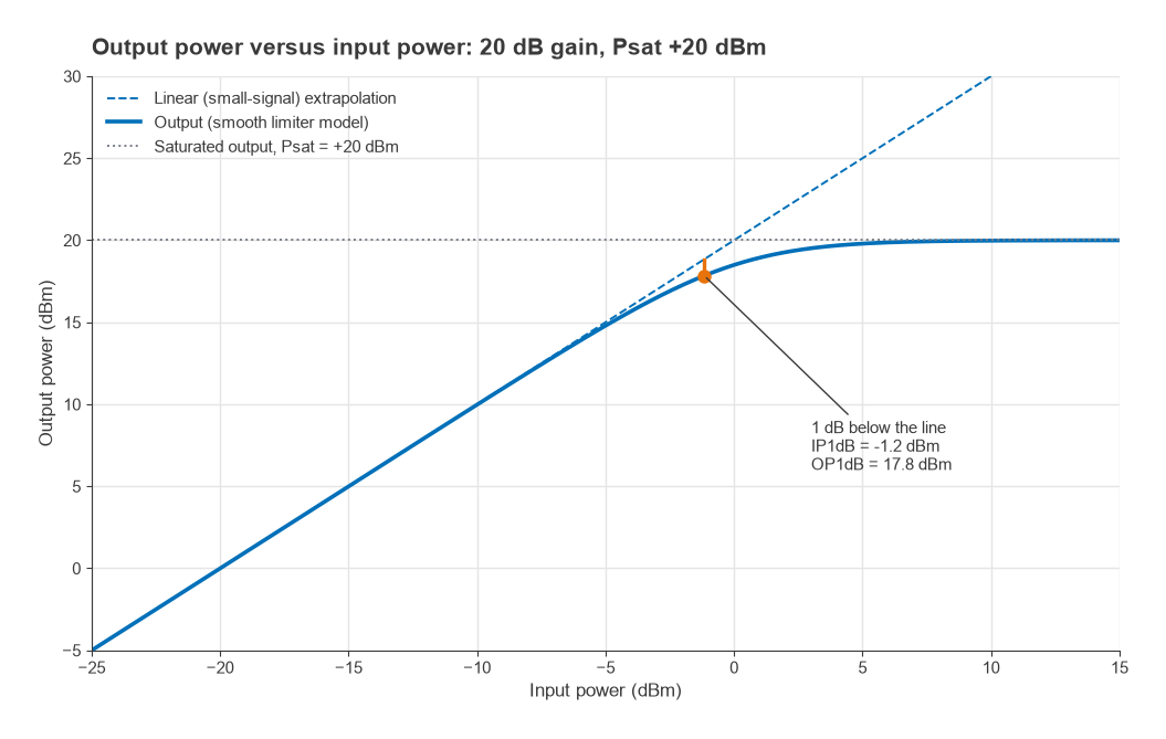
At low drive an amplifier’s output power rises one for one with input power: a 1 dB step at the input gives a 1 dB step at the output, and the gain is constant. As the drive increases, the transistor runs out of voltage swing or current, or its transconductance falls, and the output starts to lag behind the straight line. Gain compression is the difference between the straight-line (extrapolated) output and the real output. P1dB is the point where that difference reaches exactly 1 dB.
The 1 dB figure is a convention, not a physical boundary. Some power amplifier datasheets also quote P2dB or P3dB, and a few applications that need tight amplitude accuracy work to 0.1 dB compression instead. The choice of 1 dB is popular because it is large enough to measure repeatably and small enough that the amplifier is still recognisably linear.
The curve in Figure 1 comes from a smooth limiter model of an amplifier with 20 dB small-signal gain and a saturated output of +20 dBm. The 1 dB point falls at an input of −1.2 dBm and an output of +17.8 dBm, about 2.2 dB below saturation.
P1dB from the power-series model
Writing the amplifier as y = a1x + a3x3 and driving it with a single tone A cos(ωt), the output at the fundamental has amplitude
a1A + (3/4)a3A3 = a1A [1 + (3/4)(a3/a1)A2]
For a compressive device a3/a1 is negative. Setting the bracketed term equal to 10−1/20 = 0.891 gives
A1dB2 = (4/3)(1 − 0.891)|a1/a3| = 0.145 |a1/a3|
The input amplitude at the third-order intercept follows from setting the IM3 amplitude (3/4)|a3|A3 equal to a1A, which gives AIP32 = (4/3)|a1/a3|. The ratio of the two is 10log(1.333/0.145) = 9.64 dB. A device that obeys a pure cubic law therefore has its IIP3 about 9.6 dB above its IP1dB. That result is the origin of the rule of thumb discussed below.
Input P1dB Versus Output P1dB
The same point on the curve can be described by the input power that produces it or by the output power that results. At that point the actual gain is G − 1 dB, so
OP1dB = IP1dB + G − 1 (all in dB or dBm)
Convention follows the application. Power amplifiers and gain blocks are usually specified by OP1dB, because the designer cares about how much power they can deliver. Receivers, LNAs and mixers are often specified by IP1dB, because the designer cares about how large an input signal they can accept before the wanted signal is distorted or suppressed.
Worked example: converting datasheet values
- A gain block lists G = 18 dB and OP1dB = +20 dBm. Its input compression point is IP1dB = 20 − 18 + 1 = +3 dBm.
- An LNA lists G = 15 dB and IP1dB = −8 dBm. Its output compression point is OP1dB = −8 + 15 − 1 = +6 dBm.
- If the LNA is followed by a 10 dB attenuator and a mixer with IP1dB = 0 dBm, the mixer compresses when the LNA output reaches +10 dBm, which is above the LNA’s own OP1dB. The LNA compresses first, and the chain input P1dB is close to −8 dBm.
The last case shows the general rule for cascades: refer each stage’s P1dB to the chain input by subtracting the gain ahead of it, and the lowest result is a first estimate of the chain’s input P1dB. When two stages compress at similar levels the chain compresses a little earlier than either alone, so the estimate is optimistic by a fraction of a dB.
Saturated Output Power (Psat) Versus P1dB
Saturated output power, Psat, is the maximum output the amplifier can deliver however hard it is driven. Beyond P1dB the gain keeps falling until the output curve flattens. How quickly that happens depends on how sharp the knee of the transfer curve is, which in turn depends on device technology, bias class and matching.
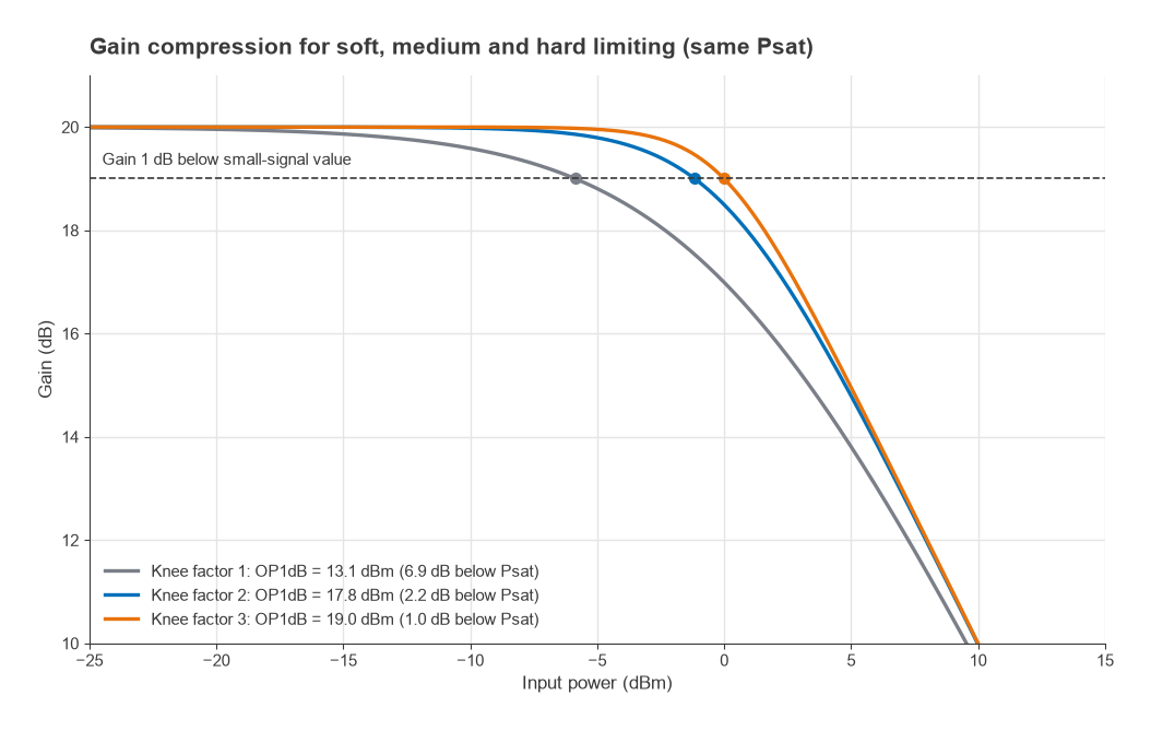
Figure 2 shows three amplifiers with identical 20 dB gain and identical +20 dBm Psat, differing only in the sharpness of the knee. The soft limiter compresses early, with OP1dB 6.9 dB below Psat. The medium case sits 2.2 dB below, and the hard limiter only 1.0 dB below. For class-A and class-AB amplifiers the gap is commonly in the range of roughly 1 to 3 dB, which is why datasheets that list both values usually show them close together. Saturated operation is acceptable for constant-envelope signals such as FM or GMSK, and is where the efficient amplifier classes described in Power Amplifier Classes and Efficiency are designed to run.
For signals with a varying envelope, Psat is not a usable operating point. The peaks are flattened, the constellation shrinks at its outer points, and spectral regrowth spills into neighbouring channels. The average power must then be backed off from P1dB by roughly the signal’s peak-to-average power ratio. An OFDM signal with a PAPR of about 10 dB on an amplifier with OP1dB = +20 dBm leaves an average output near +10 dBm unless the PA is linearized, as described in PA Linearization.
How P1dB Relates to IP3
P1dB and the third-order intercept are both set by the same curvature of the transfer function, so they move together. The power-series result above gives IIP3 ≈ IP1dB + 9.6 dB. Referred to the output, the extra 1 dB in the OP1dB definition adds to the gap:
OIP3 − OP1dB = 9.64 + 1 = 10.64 dB (pure third-order nonlinearity)
In practice engineers use the approximate rule OIP3 ≈ OP1dB + 10 dB. Real amplifiers deviate from it because higher-order terms, bias shifts and feedback all affect compression and intermodulation differently. Values from roughly 8 dB to 15 dB above OP1dB are commonly seen on datasheets. Treat the rule as a starting estimate when a datasheet lists only one of the two numbers, never as a substitute for a two-tone measurement.
Worked example: estimating intermodulation from P1dB
An amplifier has OP1dB = +20 dBm and no IP3 on its datasheet. The rule of thumb gives OIP3 ≈ +30 dBm. With two output tones of +5 dBm each, the IM3 products are
PIM3 = 3Pout − 2·OIP3 = 3(5) − 2(30) = −45 dBm
That is 50 dBc below each tone. If the real OIP3 turned out to be +27 dBm, the products would rise by 6 dB to −39 dBm, a reminder that every 1 dB of error in the intercept estimate becomes 2 dB of error in the IM3 level. The full treatment of intercept points is in Intermodulation and Intercept Points, and the way intercepts combine across stages is covered in Cascaded IP3 and System Linearity.
Measuring P1dB
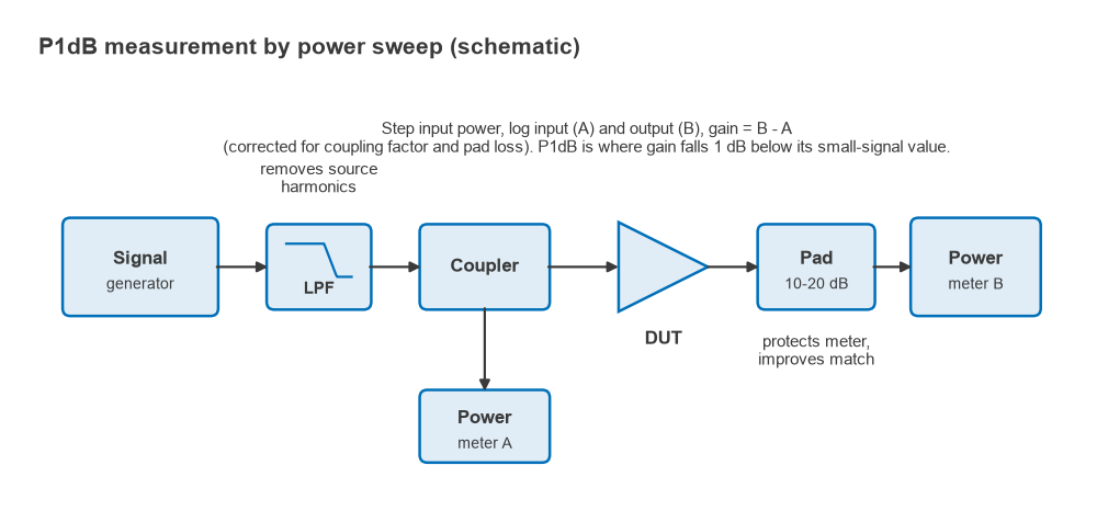
P1dB is found with a power sweep. A signal generator drives the device under test through a coupler or a characterised path, power meters or a spectrum analyzer record input and output, and the input is stepped from well below compression to a few dB beyond it. Gain is computed at each step and compared with the small-signal gain measured at the lowest levels. Many vector network analyzers automate the same sweep and report gain compression directly.
- Establish the small-signal gain at least 10 to 15 dB below the expected compression point, where the gain has stopped changing.
- Use steps of 0.5 dB or smaller near the knee, and interpolate between the two steps that bracket the 1 dB drop.
- Make sure the source chain is not itself compressing. A driver amplifier used to reach high levels needs its own P1dB well above the DUT’s IP1dB plus the path loss.
- Filter source harmonics, especially for broadband devices, or a power meter will read harmonic power as fundamental.
- Allow for heating. Pulsed and continuous-wave measurements of the same power device can differ by a fraction of a dB to more than 1 dB because junction temperature changes the gain.
Bias also matters. A class-AB amplifier’s supply current rises with drive, and a weak supply or a resistive bias feed can sag enough to move P1dB by more than the measurement uncertainty. Measure with the bias network that will be used in the product.
Using P1dB in Design
In a transmitter, OP1dB of the final stage and of each driver sets how much average power the chain can deliver for a given modulation, once PAPR backoff is applied. In a receiver, IP1dB marks the input level at which a strong wanted or unwanted signal starts to reduce the gain for everything else, which leads to the blocking and desensitization effects covered in Blocking, Desensitization and Reciprocal Mixing. The span from the noise floor to P1dB is one common definition of linear dynamic range, a narrower span than spurious-free dynamic range but easier to measure.
When selecting parts, compare P1dB with the largest signal the stage will see, including interferers, not only the wanted signal. The selection guides for low-noise amplifiers and broadband gain blocks show how P1dB is weighed against noise figure, gain and supply power.
Frequently asked questions
What is P1dB?
P1dB is the power level at which an amplifier’s gain is 1 dB lower than its small-signal gain. It marks the onset of significant gain compression and is quoted in dBm, either at the input or at the output.
What is the difference between input and output P1dB?
They describe the same point on the transfer curve. Input P1dB is the drive level that causes 1 dB of compression, and output P1dB is the power delivered at that point. They differ by the gain minus 1 dB: OP1dB = IP1dB + G − 1.
How does P1dB relate to IP3?
For a pure third-order nonlinearity, IIP3 is 9.6 dB above IP1dB and OIP3 is about 10.6 dB above OP1dB. The working rule OIP3 ≈ OP1dB + 10 dB comes from this, but real devices vary by several dB, so a measured IP3 should be used whenever one is available.
Is P1dB the same as maximum output power?
No. The maximum, or saturated, output power Psat is higher, commonly by roughly 1 to 3 dB for linear amplifier classes. Operating near Psat is acceptable for constant-envelope signals but causes severe distortion for amplitude-modulated ones.
Related topics
P1dB belongs to the linearity and distortion branch of the RF design reference. Continue with intermodulation and intercept points for two-tone behaviour, cascaded IP3 for multi-stage chains, and the RF amplifiers hub for how compression figures appear alongside the other datasheet specifications.