

kTB is the thermal noise power that a resistor at absolute temperature T delivers to a matched load in a bandwidth B, where k is Boltzmann’s constant. At the standard reference temperature of 290 K it works out to −174 dBm in each hertz of bandwidth, which is the starting point for every receiver noise floor, sensitivity and link budget calculation in RF design.
Thermal noise, also called Johnson-Nyquist noise, comes from the random motion of charge carriers in any conductor above absolute zero. It cannot be filtered out of the signal band or designed away, only reduced by narrowing the bandwidth or cooling the source. This page derives the −174 dBm/Hz figure, shows how the noise floor scales with bandwidth and noise figure, and explains why the bandwidth in the formula is the noise bandwidth rather than the 3 dB bandwidth. It is part of the noise in RF systems section.
Where Thermal Noise Comes From
Electrons in a resistor are in constant thermal agitation. At any instant there are slightly more moving one way than the other, so a small random voltage appears across the terminals. Its spectrum is flat, or white, from very low frequencies to well beyond the microwave range, and its amplitude distribution is Gaussian. Nyquist showed in 1928 that the open-circuit mean-square noise voltage of a resistance R is
vn2 = 4kTRB
where k = 1.380649 × 10⁻²³ J/K, T is the physical temperature in kelvin and B is the bandwidth in hertz. The noisy resistor can be modelled as a noiseless resistor in series with this voltage source.
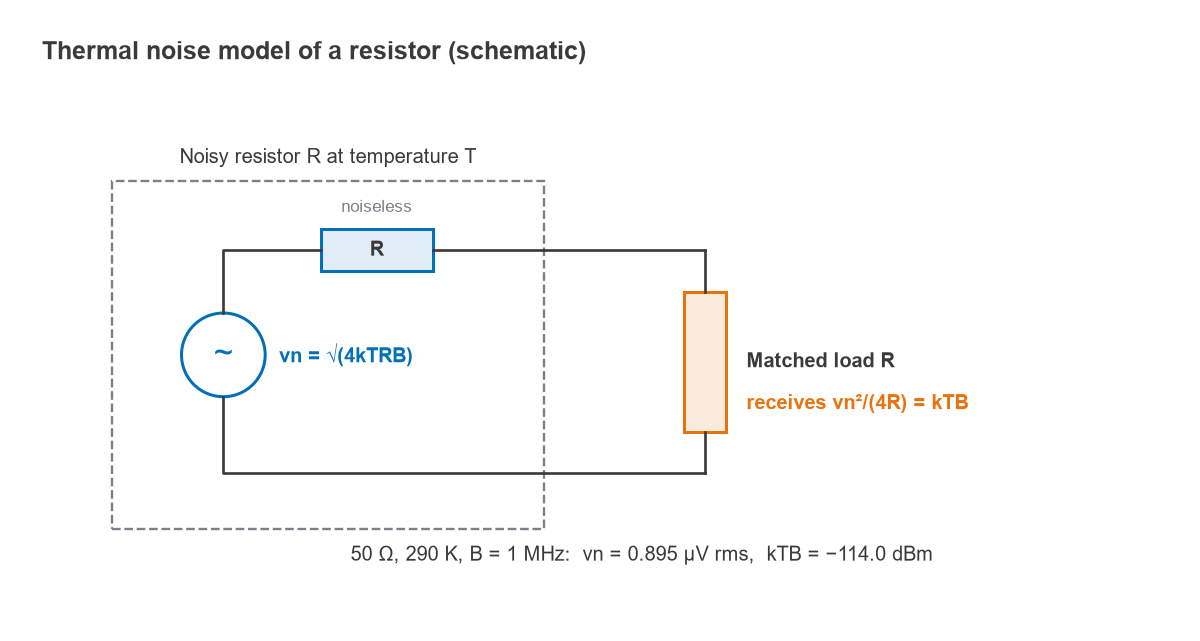
For a 50 Ω resistor at 290 K in a 1 MHz bandwidth, vn = √(4 × 1.380649 × 10−23 × 290 × 50 × 106) = 0.895 µV rms. A 1 kΩ resistor in the same bandwidth produces 4.0 µV rms. The voltage depends on R, but the power that can be extracted does not, which is why RF engineers work in power.
Available Noise Power: N = kTB
Maximum power transfer occurs when the load equals R. The noise voltage then divides equally between source and load, so the load sees vn/2 and absorbs
N = (vn/2)2 / R = 4kTRB / (4R) = kTB
R cancels. Every matched resistive source at the same temperature delivers the same available noise power, whether it is a 50 Ω termination, a 75 Ω cable or the radiation resistance of an antenna looking at 290 K ground. The density kT, in watts per hertz, is the natural unit of noise in RF work.
Why the Noise Floor Is −174 dBm/Hz
The IEEE definition of noise figure uses a reference temperature T0 = 290 K, roughly the temperature of a room or of the ground seen by a terrestrial antenna. At that temperature:
- kT0 = 1.380649 × 10−23 × 290 = 4.004 × 10⁻²¹ W/Hz.
- In dBW/Hz: 10 log(4.004 × 10⁻²¹) = −203.98 dBW/Hz.
- Adding 30 dB to convert to milliwatts: −173.98 dBm/Hz, rounded to −174 dBm/Hz.
The number depends on temperature, but only weakly in decibels. At 300 K the density is −173.83 dBm/Hz and at 358 K (85 °C) it is −173.06 dBm/Hz. A source cooled in liquid nitrogen to 77 K gives −179.73 dBm/Hz. Most link budgets simply use −174 dBm/Hz and account for real temperatures through noise temperature where it matters, as in satellite and radio astronomy receivers. The dBm conversion is the only arithmetic involved.
The kTB formula is the low-frequency limit of Planck’s law. The quantum correction becomes significant only when hf approaches kT, which at 290 K corresponds to several terahertz, so it can be ignored for practically all RF and microwave work at room temperature.
How Bandwidth Sets the Noise Floor
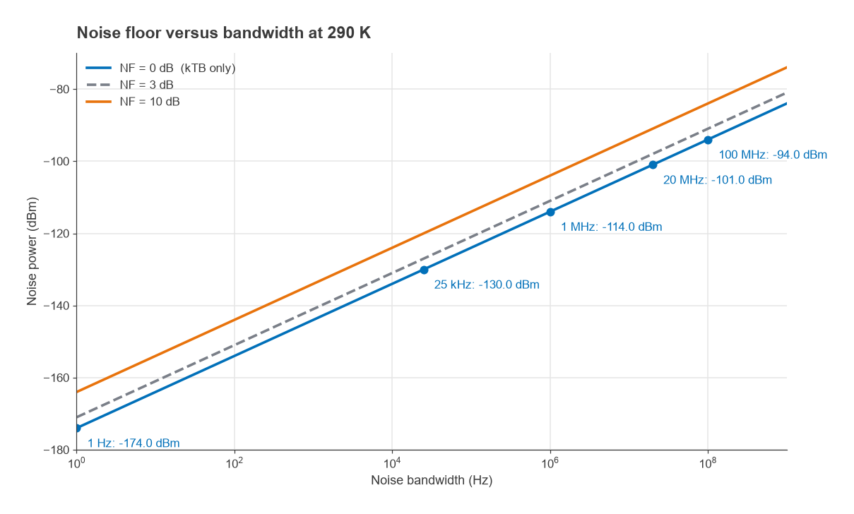
Because the density is flat, total noise power rises in proportion to bandwidth. In decibels, every factor of 10 in bandwidth adds 10 dB of noise. Adding the receiver’s noise figure gives the noise floor referred to the input:
Noise floor (dBm) = −174 + 10 log10(B) + NF
The table lists reference values at 290 K with NF = 0 dB.
| Noise bandwidth | 10 log B (dB) | kTB (dBm) |
|---|---|---|
| 1 Hz | 0 | −174.0 |
| 10 kHz | 40.0 | −134.0 |
| 25 kHz | 44.0 | −130.0 |
| 200 kHz | 53.0 | −121.0 |
| 1 MHz | 60.0 | −114.0 |
| 5 MHz | 67.0 | −107.0 |
| 20 MHz | 73.0 | −101.0 |
| 100 MHz | 80.0 | −94.0 |
Worked example: a 20 MHz channel
A receiver processes a 20 MHz wide channel and has a cascaded noise figure of 5 dB.
- 10 log(20 × 106) = 73.01 dB.
- kTB = −173.98 + 73.01 = −100.97 dBm.
- Noise floor = −100.97 + 5 = −95.97 dBm, or about −96 dBm.
If the demodulator needs 10 dB SNR, the input signal must be at least −86 dBm. That last step, adding the required SNR, is the definition of receiver sensitivity. A narrowband 125 kHz channel with a 6 dB noise figure has a floor of −174 + 50.97 + 6 = −117.0 dBm, which is one reason narrowband IoT links reach so far. The same arithmetic runs through every RF link budget.
Noise Bandwidth Versus 3 dB Bandwidth
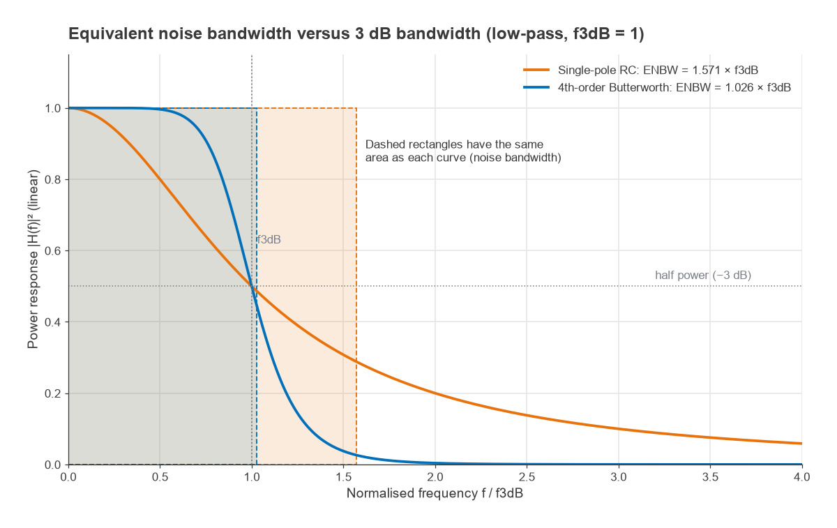
The B in kTB is the equivalent noise bandwidth (ENBW): the width of an ideal rectangular filter that passes the same total noise power as the real filter, with the same peak gain. For a power response |H(f)|2 normalised to 1 at its peak,
Bn = ∫0∞ |H(f)|2 df
Real filters have skirts, and the noise passed in those skirts counts. For an n-th order Butterworth low-pass response, the integral gives Bn / f3dB = (π/2n) / sin(π/2n). The table compares common cases.
| Filter | ENBW / 3 dB bandwidth | Noise penalty if 3 dB bandwidth is used |
|---|---|---|
| Single-pole RC | 1.571 (π/2) | 1.96 dB |
| 2nd-order Butterworth | 1.111 | 0.46 dB |
| 3rd-order Butterworth | 1.047 | 0.20 dB |
| 4th-order Butterworth | 1.026 | 0.11 dB |
| Ideal brick-wall | 1.000 | 0 dB |
For the selective channel filters used in most receivers the difference is a fraction of a decibel, and using the 3 dB bandwidth is an acceptable approximation. For a single-pole response, such as an RC-filtered detector or a simple video bandwidth, the error approaches 2 dB and should not be ignored. Spectrum analyzer resolution bandwidth filters also have an ENBW that differs from the nominal RBW; the analyzer’s documentation usually gives the ratio, and the spectrum analyzer basics page explains how it enters noise measurements.
For a bandpass filter the same idea applies with the integral taken across the passband: the noise bandwidth of a channel is roughly its channel filter’s ENBW, not its RF bandwidth, which is why the baseband or IF filter sets the noise floor of a superheterodyne receiver.
From kTB to System Noise
kTB is the noise of an ideal matched source. Every active and lossy stage after it adds more, and the noise figure describes how much. In terms of noise temperature, a receiver with equivalent input noise temperature Te sees a total input-referred noise of k(TA + Te)B, where TA is the antenna or source temperature. When TA = T0 = 290 K this reduces to the familiar −174 + 10 log B + NF. When the antenna looks at cold sky, TA may be far below 290 K and the receiver’s own noise dominates, which is why satellite ground stations specify LNAs by noise temperature rather than noise figure.
Stages in cascade add noise according to the Friis formula for cascaded noise figure, which is why the first stage of a receiver, normally the low noise amplifier, matters most.
Frequently Asked Questions
What is kTB?
kTB is the available thermal noise power from a resistive source, the product of Boltzmann’s constant, absolute temperature and bandwidth. It is the minimum noise any matched receiver at that source temperature must accept. At 290 K it is −174 dBm in 1 Hz and −114 dBm in 1 MHz.
Why is the noise floor −174 dBm/Hz?
Because kT at the reference temperature of 290 K equals 4.0 × 10⁻²¹ W/Hz, which is −204 dBW/Hz or −174 dBm/Hz. The value is a convention tied to that reference temperature. At other source temperatures it shifts slightly, by about 0.15 dB between 290 K and 300 K.
How does bandwidth affect noise?
Thermal noise power is proportional to bandwidth, so the noise floor rises by 10 log of the bandwidth ratio. Doubling the bandwidth adds 3 dB and a tenfold increase adds 10 dB. This is why narrowband receivers achieve better sensitivity than wideband ones with the same noise figure.
Does thermal noise depend on the resistor value?
The open-circuit noise voltage does, as √(4kTRB). The available noise power, kTB, does not, because a larger resistance produces more voltage but delivers it into a correspondingly larger matched load.
Related Topics
Continue with noise figure and noise factor, noise temperature and cascaded noise figure, then see how the noise floor turns into a sensitivity number in Radio Architectures Part 4. The RF design overview places noise alongside linearity, matching and the other core topics.