

Part 15, Link Budgets, Putting the Radio Together, closed a 10 km link with about 25 dB of margin. One line in that budget was taken on trust: the 10 dB of signal-to-noise ratio the demodulator was assumed to need. That number is not a property of the hardware. It is set by the modulation, by the error rate the system will accept, and by how much distortion the transmitter and receiver add on top of thermal noise.
This part opens up that line. It covers how symbols are mapped onto a carrier, how much SNR each modulation order needs, how error vector magnitude (EVM) measures the quality of a real signal, and why the peak-to-average power ratio (PAPR) of the waveform has so much influence on the power amplifier choices made in Part 7 and Part 8.
From Bits to Symbols: Constellations and Bandwidth
A digital transmitter groups bits into symbols and maps each symbol to a point in the I/Q plane. With M points in the constellation, each symbol carries log2M bits. QPSK has 4 points and 2 bits per symbol, 16-QAM has 16 points and 4 bits, 64-QAM carries 6 bits and 256-QAM carries 8. Square QAM constellations are almost always Gray coded, so that the nearest neighbours of any point differ by a single bit. A symbol error caused by noise then usually costs only one bit.
The symbols are sent at a symbol rate Rs, and each one is shaped by a pulse-shaping filter so that the spectrum is contained. The usual choice is a root-raised-cosine (RRC) filter, split between transmitter and receiver so that the cascade is a raised cosine with no intersymbol interference at the sampling instants. The occupied bandwidth is
B = Rs(1 + α)
where α is the roll-off factor, typically between 0.1 and 0.35. A 20 Msymbol/s carrier with α = 0.22 occupies 20 × 1.22 = 24.4 MHz. With 256-QAM, the same carrier carries 20 × 8 = 160 Mb/s before coding. Moving from QPSK to 256-QAM quadruples the raw bit rate in the same bandwidth, and the price is paid in SNR.
OFDM, used in LTE, 5G NR and Wi-Fi, reaches the same goal differently. It divides the channel into many narrow subcarriers, each carrying its own QAM symbol at a low rate. The individual subcarriers are still QAM, so the SNR requirements below still apply, but the sum of many subcarriers has very different peak statistics from a single carrier.
How Much SNR Each Modulation Needs
For square M-QAM in additive white Gaussian noise, the symbol error probability is
Ps = 1 − (1 − P√M)2, with P√M = 2(1 − 1/√M) Q(√(3Es/((M − 1)N0)))
where Es/N0 is the symbol energy to noise density ratio and Q is the Gaussian tail function. When the receiver uses a filter matched to the RRC pulse, the noise bandwidth equals the symbol rate and Es/N0 is the same as the SNR used in the sensitivity equation of Part 4. The energy per bit follows from Eb/N0 = Es/N0 − 10log(log2M).
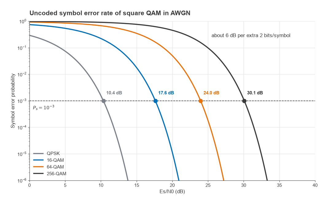
Solving the expression numerically for an uncoded symbol error rate of 10−3 gives the following.
| Modulation | Bits per symbol | Es/N0 for Ps = 10−3 | Eb/N0 |
|---|---|---|---|
| QPSK | 2 | 10.4 dB | 7.3 dB |
| 16-QAM | 4 | 17.6 dB | 11.6 dB |
| 64-QAM | 6 | 24.0 dB | 16.2 dB |
| 256-QAM | 8 | 30.1 dB | 21.1 dB |
Each step from 16-QAM upward adds 2 bits per symbol and costs about 6 dB, because the constellation spacing halves for the same average power. Forward error correction lowers all of these figures by several dB, and real systems quote their requirement at a coded block error rate rather than an uncoded symbol error rate, but the 6 dB per step remains. A system with adaptive modulation picks the highest order the current SNR supports, which is why a link with spare margin turns it into throughput rather than leaving it unused.
The 10 dB assumed in Part 15 is therefore roughly what an uncoded QPSK link needs at a 10−3 symbol error rate. Running the same link at 256-QAM would consume about 20 dB of its 25 dB margin.
Error Vector Magnitude
Thermal noise is not the only thing that moves a received symbol away from its ideal position. Phase noise rotates it, I/Q imbalance distorts the constellation, PA compression pulls in the outer points and DAC quantization adds its own noise. EVM lumps all of these together. For each symbol, the error vector is the difference between the measured point and the ideal reference point, and
EVMrms = √( mean|ek|2 / mean|sk|2 )
where ek is the error vector and sk the reference symbol. It is quoted in percent or in dB as 20log(EVM). Most modern standards normalize to the average constellation power as written here. Some older ones normalize to the peak constellation point, which gives a smaller number for the same signal, so the definition must be checked before comparing figures from different sources.
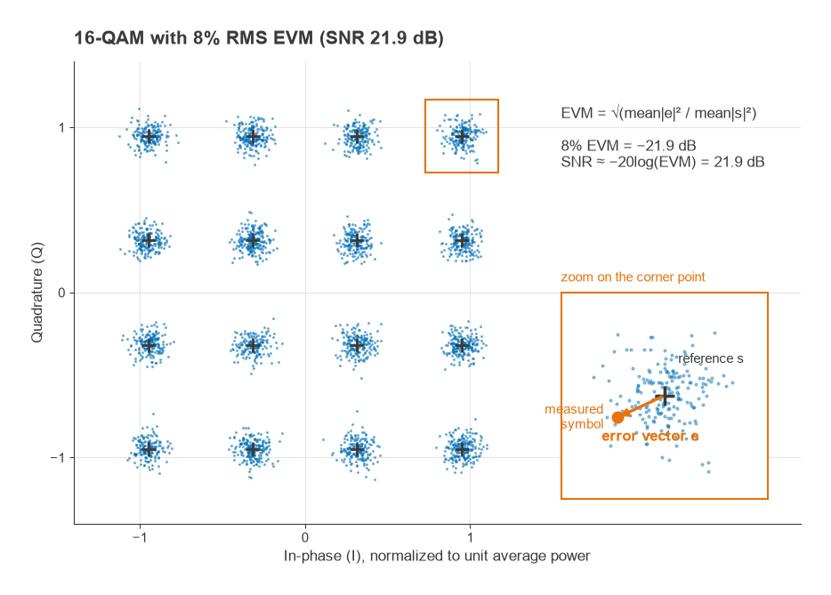
When the error is noise-like, EVM and SNR are two views of the same quantity:
SNR ≈ −20log(EVMrms)
An EVM of 8% corresponds to an SNR of 21.9 dB, and 3.5% corresponds to 29.1 dB. This is why EVM limits in a standard step down with modulation order. The 3GPP NR base station specification, for example, allows 17.5% for QPSK, 12.5% for 16-QAM, 8% for 64-QAM and 3.5% for 256-QAM. Converted to dB, those limits are −15.1, −18.1, −21.9 and −29.1 dB, and each sits comfortably above the uncoded requirements in the table, leaving room for the receiver’s own noise.
The relationship also shows how a transmitter and receiver share the error budget. Because independent error sources add in power, a transmitter at 3.5% EVM (an SNR of 29.1 dB) received at a thermal SNR of 30 dB gives an effective SNR of
SNReff = −10log(10−2.912 + 10−3.0) = −10log(0.001225 + 0.001000) = 26.5 dB
equivalent to 4.7% EVM. The receiver sees a signal worse than either the transmitter or its own front end alone. Part 6 built the transmitter half of this budget as a root-sum-square of image, phase noise, LO leakage and PA contributions. The same arithmetic extends across the link.
EVM has limits as a metric. It treats all error as if it were noise, so a deterministic distortion such as AM/AM compression of the outer points is reported as a single RMS number even though it hits only some symbols. Measurement standards also define which corrections, such as equalization of a linear frequency response tilt, are applied before EVM is computed.
Peak-to-Average Power Ratio
PAPR is the ratio of the peak instantaneous envelope power of a signal to its average power. It is usually defined on the complex envelope, so an unmodulated carrier has a PAPR of 0 dB. Defined on the RF waveform itself, a sine wave has a peak-to-average ratio of 3 dB, and the two conventions differ by that amount. This page uses the envelope definition, as most instruments do.
The constellation alone sets a floor. For square M-QAM with levels ±1, ±3 and so on, the average symbol power is 2(M − 1)/3 and the corner point has power 2(√M − 1)2:
- 16-QAM: 18/10, or 2.55 dB.
- 64-QAM: 98/42, or 3.68 dB.
- 256-QAM: 450/170, or 4.23 dB.
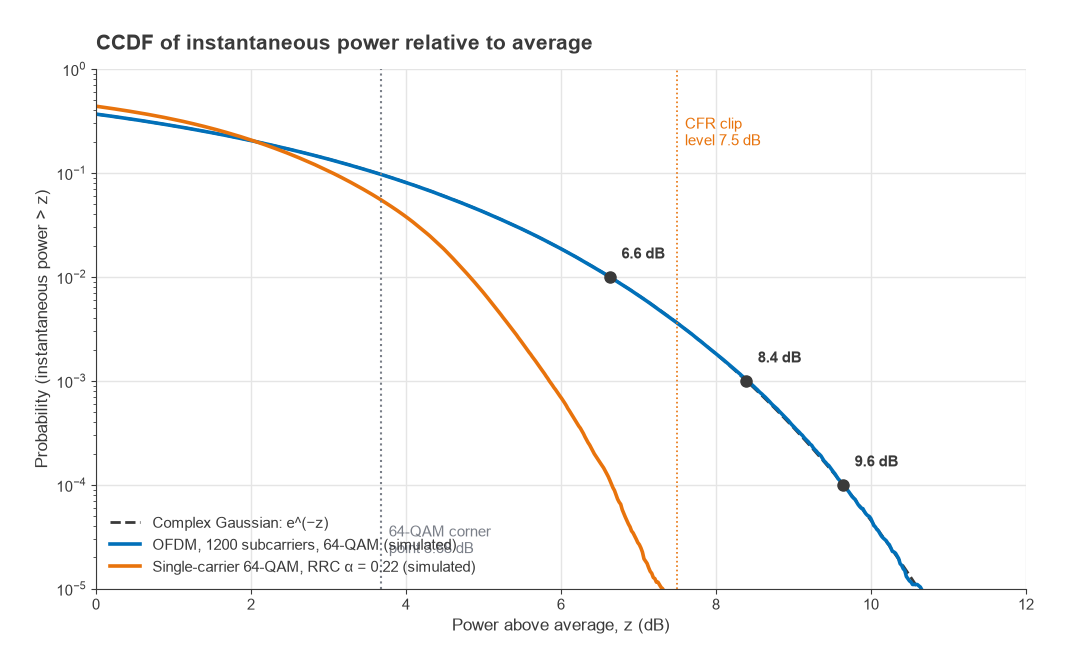
Pulse shaping adds to this. Between sampling instants, the RRC filter output is a weighted sum of several neighbouring symbols, and when they line up the envelope overshoots the corner points. Smaller roll-off factors give longer impulse responses and larger overshoots. A simulation of single-carrier 64-QAM with α = 0.22 reaches about 6.7 dB at the 0.01% probability point, roughly 3 dB above its constellation value.
OFDM is worse. Its time-domain signal is the sum of hundreds or thousands of independently modulated subcarriers, and by the central limit theorem the I and Q samples approach Gaussian distributions. The envelope is then Rayleigh distributed and the instantaneous power is exponentially distributed. The probability that the instantaneous power exceeds z times the average is
P(Pinst > z Pavg) = e−z
With no hard peak, OFDM PAPR is quoted at a probability on the complementary cumulative distribution function (CCDF). Setting e−z = 10−4 gives z = 9.21, or 9.6 dB. At 0.1% the figure is 8.4 dB and at 1% it is 6.6 dB. An unclipped OFDM signal therefore needs close to 10 dB of headroom above its average power if peaks occurring 0.01% of the time are to pass undistorted.
Worked Example: Headroom, Clipping and PA Power
Take an OFDM transmitter whose PA saturates at +46 dBm (about 40 W). To pass peaks at the 0.01% CCDF point, the average output must sit 9.6 dB below saturation:
Pavg = 46 − 9.6 = +36.4 dBm, or 4.4 W
Crest factor reduction, introduced in Part 7, clips the envelope digitally before the DAC. Suppose the signal is clipped at 7.5 dB above its average power. For a complex Gaussian signal clipped in magnitude at a level γ times the average power, the output can be split into a scaled copy of the input, αx, plus an uncorrelated distortion term. The scale factor and distortion power are
α = 1 − e−γ + (√(πγ)/2) erfc(√γ)
Pd = (1 − e−γ) − α2
With γ = 100.75 = 5.62, α = 0.998 and Pd = 2.56 × 10⁻⁴, giving an EVM contribution of √Pd/α = 1.6%, or about −35.9 dB. Clipping at 6 dB instead raises it to 4.1%. Both results agree with a direct simulation of a clipped Gaussian signal. These figures cover clipping alone. A practical CFR stage must also filter the clipping noise out of the adjacent channels, which regrows some of the peaks and moves part of the distortion in-band, so the final EVM cost is somewhat higher.
With the PAPR held to 7.5 dB, the average output becomes
Pavg = 46 − 7.5 = +38.5 dBm, or 7.1 W
The 2.1 dB reduction in headroom is a factor of 1.62 in average power from the same device. Put the other way, the same 4.4 W average could be delivered by a PA rated 2.1 dB lower, which runs closer to its efficient region for the same output. A 1.6% EVM contribution is small against a 3.5% limit for 256-QAM, but it still has to be added in power to the PA, phase noise and DAC terms already in the budget. This trade between headroom, efficiency and EVM is the reason CFR, DPD and Doherty amplifiers appear together in nearly every modern high-power transmitter.
Whatever clipping or compression remains also spreads energy outside the channel. The adjacent channel leakage ratio (ACLR), the power in the adjacent channel relative to the wanted channel, is the out-of-band counterpart of EVM. Third-order distortion of a signal with bandwidth B produces regrowth spanning about 3B, extending a full channel width either side of the wanted signal, so it falls directly into the neighbouring channels. At low modulation orders the constellation tolerates a lot of in-band error and ACLR tends to set the back-off. At high orders the EVM limit is tight enough that it often sets the back-off instead.
Next in the Series
The modulation sets how much SNR the link needs. The antennas and the path decide how much it gets. Part 17, Antennas and Propagation for Radio Designers, looks at gain, aperture, beamwidth and polarization from the radio designer’s side, and at how real paths depart from the free-space loss used in Part 15.