

Part 10 of this series, Frequency Synthesis, PLLs and Phase Noise, dealt with the local oscillator: how a PLL produces a clean carrier and how its phase noise spreads into neighbouring channels. That oscillator has a close relative in every modern transmitter, the sample clock of the digital-to-analog converter. The quality of that clock, and of the converter it drives, sets a floor under everything the transmitter does afterwards.
Part 5 covered ADCs and receivers. The DAC is the mirror image of that problem. Instead of turning a continuous waveform into numbers, it turns numbers into a staircase of voltages or currents, and the transmit chain behind it has to smooth, translate and amplify that staircase without adding much of its own damage. This part looks at what the DAC actually produces, how its imperfections show up in the spectrum, and how the analog chain between DAC and power amplifier is planned.
What a DAC Really Outputs
Most high-speed RF DACs are current-steering designs. An array of switched current sources is weighted, usually with the most significant bits thermometer-coded and the lower bits binary-weighted, and the switches are steered into a differential load on each clock edge. The output holds its value for one full clock period and then jumps to the next value. This is called non-return-to-zero (NRZ) or zero-order hold operation.
Holding a value for a full period is the same as convolving the ideal impulse train with a rectangular pulse of width Ts = 1/fs. In the frequency domain that pulse becomes a sinc envelope:
H(f) = sin(πf/fs) / (πf/fs)
Two consequences follow. First, the wanted signal in the first Nyquist zone is attenuated more as it approaches fs/2, where the droop reaches 20log(2/π) ≈ −3.92 dB. Second, the sampled spectrum repeats around every multiple of fs, so images appear at fs − fout, fs + fout, 2fs − fout and so on. The sinc envelope reduces those images but does not remove them, and it has nulls at every integer multiple of fs.
Worked example: sinc droop and the first image
Take a DAC clocked at fs = 1 GSPS producing a tone at fout = 350 MHz.
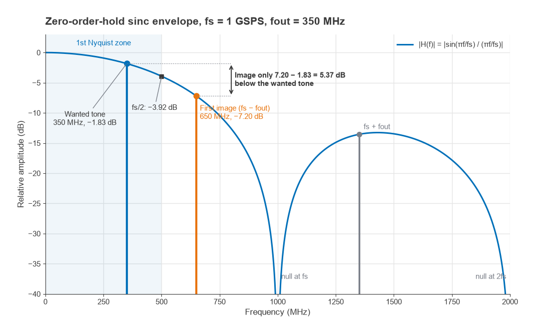
- At 350 MHz, f/fs = 0.35. sin(0.35π) / (0.35π) = 0.8910 / 1.0996 = 0.8103, or −1.83 dB.
- The first image sits at 1000 − 350 = 650 MHz. There f/fs = 0.65, and sin(0.65π) / (0.65π) = 0.8910 / 2.0420 = 0.4363, or −7.20 dB.
- The image is therefore only 7.20 − 1.83 = 5.37 dB below the wanted tone.
A 5 dB separation is nowhere near enough for a transmitter that must meet a spurious emission mask. If the system needs the image 70 dB down at the antenna, the reconstruction filter has to supply roughly 65 dB of rejection at 650 MHz while passing 350 MHz with little loss and flat group delay. That is a demanding filter, which is why designers rarely run a DAC this close to Nyquist without help from interpolation.
Resolution, Noise Spectral Density and Spurs
The ideal quantization-limited SNR of an N-bit converter for a full-scale sine wave is the familiar
SNR = 6.02N + 1.76 dB
That noise is spread across the Nyquist band, 0 to fs/2. For RF work the more useful figure is noise spectral density (NSD), the noise per hertz relative to full scale:
NSD = −SNR − 10log(fs/2) dBFS/Hz
For an ideal 14-bit DAC at 1 GSPS, SNR = 6.02 × 14 + 1.76 = 86.04 dB, and 10log(500 × 106) = 86.99 dB, so the quantization NSD is about −173.0 dBFS/Hz. Real parts never get there. Thermal noise in the current sources, clock jitter and the output stage all add to it, and a practical DAC often lands 10 to 20 dB above the quantization limit. The lesson from the formula still holds: doubling the clock rate spreads the same total noise over twice the bandwidth and lowers the density by 3 dB, which is the processing gain the transmit side gets from oversampling.
Spurious-free dynamic range (SFDR) is a separate specification and usually the harder one. Static mismatch between current sources produces harmonic distortion. Dynamic effects, such as unequal switching times, code-dependent glitch energy and output impedance that varies with code, produce harmonics and intermodulation that typically worsen as the output frequency rises. The harmonics also fold. A 350 MHz tone at 1 GSPS has its second harmonic at 700 MHz, which images back to 1000 − 700 = 300 MHz, only 50 MHz from the carrier. Frequency planning, the same exercise done for mixers in Part 2, applies to DACs as well.
Clock Jitter on the Transmit Side
A timing error Δt on a clock edge produces an amplitude error proportional to the slope of the signal at that instant. For a sine wave at frequency f with random rms jitter tj, the jitter-limited SNR is
SNRjitter = −20log(2πf tj)
For f = 400 MHz and tj = 100 fs, 2π × 400 × 106 × 100 × 10−15 = 2.51 × 10⁻⁴, giving an SNR of 72.0 dB. That is already below the quantization limit of a 12-bit converter (74 dB), so a high-resolution DAC fed from an ordinary clock wastes its extra bits. The formula is identical to the one used for ADCs, and it explains why the sample clock is generated by a low-noise PLL or a dedicated clock cleaner of the kind described in Part 10. The integrated phase noise of that clock converts directly to tj, and the close-in part of it appears as a skirt around the carrier in exactly the way LO phase noise does.
Interpolation, Digital Upconversion and Mix Mode
The image problem in the first example came from running the DAC at only 2.86 times the output frequency. The usual fix is interpolation. Baseband I/Q samples arrive at a modest rate, digital half-band filters raise the rate by 2, 4, 8 or more, and a numerically controlled oscillator (NCO) shifts the signal to a digital IF before it reaches the converter core. Because the interpolation filters suppress the digital images before conversion, the only images left are those around multiples of the final clock rate, which are far away and easy to filter.
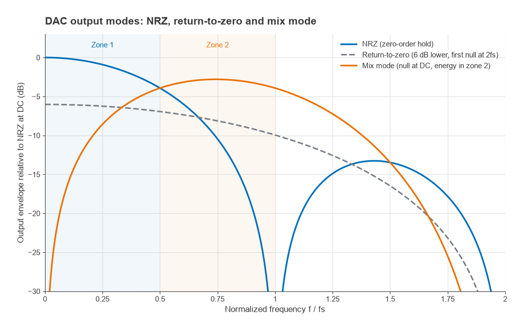
Some DACs offer alternative output modes that reshape the sinc envelope. In return-to-zero mode the output returns to zero for half of each period, which widens the main lobe of the sinc so the first null moves to 2fs. The cost is 6 dB less fundamental power. In mix mode (sometimes called RF mode) the output is inverted for the second half of each period, which puts a null at DC and pushes energy into the second Nyquist zone. That allows a deliberate image at fs − fout or fs + fout to be used as the transmitted signal, at the price of reduced first-zone output and a filter that must now select a higher-zone image. These modes are the transmit-side counterpart of the undersampling techniques covered in Part 13.
Building the Analog Transmit Chain
After the DAC there are two common arrangements. In a direct-conversion transmitter, a pair of baseband or low-IF DACs drives an I/Q modulator, which translates the signal to RF using a quadrature LO. In an RF-DAC or direct-synthesis transmitter, the DAC output is already at the carrier frequency and only filtering and gain stages follow. Either way, the chain between converter and PA typically contains:
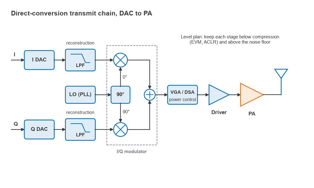
- A reconstruction or anti-image filter, sized by the image calculation above.
- A balun or transformer if the DAC output is differential and the following stage is single-ended.
- An I/Q modulator, for the direct-conversion case, whose LO leakage and quadrature errors produce a carrier spur and an image sideband. Part 12 treats those errors in detail for the receive side; the arithmetic is the same.
- A variable-gain amplifier or digital step attenuator for power control.
- One or more driver amplifiers that bring the level up to what the PA needs.
The level plan has two competing goals. The signal must stay far enough below each stage’s compression point to preserve EVM and adjacent channel leakage, which matters a great deal with high peak-to-average signals such as OFDM. At the same time it must stay far enough above the noise floor that the chain does not swamp a receiver in the transmitter’s own duplex band or in a co-located radio. The DAC is often run with its rms level 12 to 15 dB below full scale to leave headroom for peaks, and that backoff costs SNR one dB for one dB.
Worked example: output noise floor
Suppose a DAC has a full-scale output of −2 dBm and a measured NSD of −160 dBFS/Hz at the frequency of interest. Its absolute noise density is then −2 − 160 = −162 dBm/Hz. The chain that follows has 40 dB of gain to the PA input and a cascaded noise figure of 10 dB.
- DAC noise at the chain output: −162 + 40 = −122 dBm/Hz.
- Noise added by the chain itself, referred to its output: −174 + 10 + 40 = −124 dBm/Hz.
- Total: 10log(10−12.2 + 10−12.4) = −119.9 dBm/Hz.
Neither source dominates, so improving only one of them buys at most about 2 dB. If this transmitter shares an antenna with a receiver 50 MHz away, the PA will raise that noise further by its own gain, and the duplexer has to provide enough isolation to bring it below the receiver’s floor. Part 14 runs that calculation. The point here is that transmit noise is set at the very start of the chain, by the DAC and its clock, and every stage afterwards only adds to it.
A useful habit is to tabulate gain, noise figure, output compression and output noise density for each stage, just as a receiver lineup is tabulated. The transmit lineup is usually checked in the other direction: start from the required PA input level and work backwards to see how much of the DAC’s range is actually being used.
Next in the Series
The direct-conversion transmitter mentioned above has a receive-side twin that has taken over most handsets and many base stations. Part 12, Zero-IF Receivers, DC Offset and I/Q Imbalance, explains why removing the IF is attractive, and what DC offset, flicker noise, second-order distortion and quadrature errors cost in return.