Radio Architectures: The Complete 20-Part Series

A radio architecture is the arrangement of amplifiers, filters, mixers, oscillators and data converters that moves a signal between the antenna and digital baseband. The main receiver architectures are the superheterodyne, the zero-IF (direct-conversion) receiver, the low-IF receiver and the direct RF sampling receiver. They differ mainly in where the signal is translated in frequency and where it is digitised.

This page is the index to the Radio Architectures series, a 20-part walk through radio hardware for working engineers and students. Each part takes one block or one system question and works it through with formulas and numbers. The series sits within the wider RF design guide, and several parts double as the main reference pages for their topic on this site.

The Main Receiver Architectures

Every receiver has to do three things: select the wanted channel, raise it far enough above the noise and distortion of later stages, and present it to an analog-to-digital converter in a form that converter can handle. The architectures trade analog filtering against converter speed and digital correction.

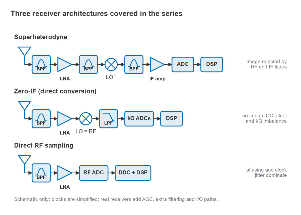
Simplified block diagrams of superheterodyne, zero-IF and direct RF sampling receivers — Figure 1: Simplified superheterodyne, zero-IF and direct RF sampling receivers (schematic only).

Superheterodyne. A mixer translates the RF signal to a fixed intermediate frequency (IF), where fixed, sharp filters select the channel. The price is an image frequency on the other side of the LO that must be filtered out before the mixer.
Zero-IF. The LO sits at the carrier frequency, so the signal lands directly at baseband as I and Q components. There is no image band to filter, but DC offset, flicker noise, second-order distortion and I/Q imbalance appear instead.
Low-IF. A compromise that places the signal at a small IF, often a channel width or two from DC, to avoid DC problems while keeping most of the integration benefits of zero-IF. The image is then an adjacent channel and is rejected by quadrature processing.
Direct RF sampling. A fast ADC digitises the RF band directly, and digital down-conversion does the rest. Analog filtering moves to anti-alias duty, and clock jitter and converter power become the limits.

The image frequency in numbers

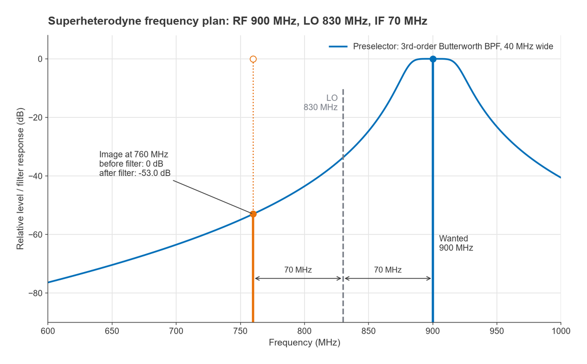
For a superheterodyne with low-side LO injection, f_LO = f_RF − f_IF and the image lies at f_image = f_RF − 2f_IF. A 900 MHz signal with a 70 MHz IF needs an 830 MHz LO, and the image sits at 900 − 140 = 760 MHz. A third-order Butterworth preselector centred on 900 MHz with a 40 MHz bandwidth attenuates 760 MHz by about 53.0 dB. If the system needs more image rejection than that, the designer can raise the IF, add filter order or move to an image-reject mixer. That trade is the central design question of Part 2.

Superheterodyne frequency plan with 900 MHz signal, 830 MHz LO and image at 760 MHz attenuated 53 dB by a preselector — Figure 2: Frequency plan for a 900 MHz signal with a 70 MHz IF. A 3rd-order Butterworth preselector attenuates the 760 MHz image by 53.0 dB.

Architecture Comparison

The table summarises the qualitative differences. The dedicated comparison page, superheterodyne vs zero-IF vs direct sampling, works through a selection example in detail.

Architecture	Where the channel is selected	Image handling	Dominant impairments	Typical fit
Superheterodyne	Fixed IF filter	RF preselector and IF choice	Image, spurs from the frequency plan, filter size	High selectivity and dynamic range, test equipment, many base stations
Zero-IF	Baseband low-pass filters	No image band; quadrature errors set residual image	DC offset, flicker noise, IP2, I/Q imbalance, LO leakage	Highly integrated transceivers, handsets
Low-IF	Complex (polyphase) filter or digital filter	Quadrature rejection of an adjacent-channel image	Image rejection limited by I/Q matching	Narrowband, low-power receivers
Direct RF sampling	Digital filters after the ADC	Anti-alias filter and frequency planning across Nyquist zones	Clock jitter, ADC spurs, converter power	Multi-band and wideband systems, SDR

The Series, Part by Part

All 20 parts are published. Some early parts sit at older addresses; the links below always point to the current page.

Understand Radio Architectures, Part 1: the starting point, introducing the blocks that make up a radio and how a signal moves through them.
Receivers, LOs and Mixers: frequency translation, LO injection and the image problem.
Intermodulation and Intercept Points: two-tone distortion, IP3 and how intercept points cascade.
Sensitivity, Noise and Front-End Amplifiers: kTB, noise figure, the Friis formula and receiver sensitivity.
ADCs and Receivers: converter resolution, sampling, SNR and where the ADC sits in the chain.
Transmitter Architectures: direct-conversion, heterodyne and polar transmitters.
Power Amplifier Classes and Efficiency: the main amplifier classes and the efficiency they trade for linearity.
PA Linearization: feedforward, digital predistortion and Doherty amplifiers.
RF Filters: filter types, specifications and their place in the signal chain.
Frequency Synthesis, PLLs and Phase Noise: how local oscillators are generated and how clean they are.
DACs and the Transmit Signal Chain: sinc droop, images, clock jitter and transmit level planning.
Zero-IF Receivers, DC Offset and I/Q Imbalance: the direct-conversion receiver and its characteristic errors.
Direct RF Sampling and Software-Defined Radio: Nyquist zones, jitter limits and digital down-conversion.
Front-End Modules, Duplexers and Switches: integrated front ends and transmit-to-receive isolation.
Link Budgets, Putting the Radio Together: path loss, margins and the complete system calculation.
Modulation, EVM and PAPR: how modulation quality and peak-to-average ratio constrain the hardware.
Antennas and Propagation for Radio Designers: antenna gain, efficiency and the propagation channel.
MIMO, Beamforming and Phased Arrays: multi-antenna hardware and its calibration.
mmWave Radio Architectures: what changes above about 24 GHz.
Measuring Radio Performance: verifying sensitivity, linearity, EVM and spectral masks on the bench.

Companion pages

Low-IF Receivers: polyphase filtering and the image-rejection budget of a low-IF design.
Superheterodyne vs Zero-IF vs Direct-Sampling: a decision guide for choosing a receiver architecture.
RF Link Budget Calculator: an interactive version of the Part 15 calculation.

Reading Paths

For students

Read Parts 1 and 2 first, then Parts 4 and 3 in that order, because sensitivity and intercept points together define dynamic range. Continue with Part 5 and Part 6 to see both directions of the radio, then Part 15 to tie everything into a link budget. The RF fundamentals and S-parameters pages fill in background as needed.

For working engineers

Go straight to the part that matches the current problem. Receiver designers usually start with Parts 12, 13 and 14; transmitter and PA designers with Parts 7, 8 and 11; synthesizer work with Part 10. Part 15 is the place to check a system-level number quickly.

Frequently Asked Questions

What are the main radio receiver architectures?

The superheterodyne, zero-IF (direct conversion), low-IF and direct RF sampling receivers. Variants such as dual-conversion superheterodynes and image-reject receivers build on the same ideas.

Superheterodyne vs zero-IF vs direct sampling: which is best?

None is best in general. The superheterodyne offers strong selectivity at the cost of filters and an image band. Zero-IF integrates well but must manage DC offset and I/Q errors. Direct sampling gives the most flexibility but demands fast converters and very low clock jitter. The right choice follows from the bandwidth, dynamic range, power and cost targets.

Do the parts need to be read in order?

No. Each part states what it assumes and links back to the earlier parts it builds on. Reading in order helps students, because later parts reuse the noise, linearity and frequency-planning results from Parts 2 to 4 without deriving them again.