Radio Architectures, Pt 19: Millimeter-Wave Radio Architectures

Part 18, MIMO, Beamforming and Phased-Array Architectures, treated arrays as a general tool: array gain, beam steering, element spacing, a choice of where in the chain the weights are applied, and spatial multiplexing for capacity. At sub-6 GHz frequencies an array is an option. Above roughly 24 GHz it stops being optional. The wavelengths are short enough that dozens of elements fit in the palm of a hand, and the path loss between isotropic antennas is high enough that a single-element radio would rarely close a useful link.

This part looks at what changes in the radio itself when the carrier moves into the millimetre-wave range. The block diagrams from earlier parts still apply: there is still an LNA, a mixer, a synthesizer and a PA. What changes is how many of each there are, where they sit relative to the antenna, and which impairments dominate.

What Changes Above 24 GHz

Strictly, millimetre waves run from 30 GHz to 300 GHz, where the free-space wavelength is between 10 mm and 1 mm. In practice the term is used more loosely for the bands now used for communications: the 5G NR FR2 range starting at 24.25 GHz, the unlicensed band around 60 GHz, and the 71 to 76 GHz and 81 to 86 GHz E-band allocations used for point-to-point backhaul.

The wavelength sets the scale of everything. At 28 GHz, λ = c/f = 10.71 mm, so half-wavelength element spacing is 5.35 mm. At 60 GHz the spacing drops to 2.50 mm. A transceiver channel for each element has to fit behind an area of that size, or be connected to it by a line short enough not to waste the signal. Three consequences follow from that one fact:

• Interconnect becomes a loss budget item measured in millimetres. A trace that would be negligible at 2 GHz can cost a meaningful fraction of a dB at 28 GHz, ahead of the LNA.
• The antenna and the RF electronics tend to merge. Antenna-in-package designs place the elements directly above the beamformer ICs.
• Connectorized testing becomes the exception. Many arrays have no RF port at all, which shapes the measurement methods in Part 20.

Path Loss, Aperture and the Atmosphere

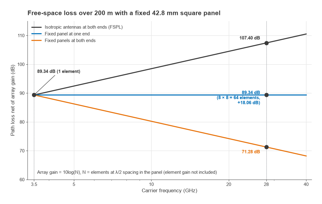
Part 15 noted that the frequency term in free-space path loss belongs to the isotropic antenna, not to the air, and Part 17 tied antenna gain to aperture area. Millimetre-wave design is where that distinction pays off. The effective aperture of an isotropic antenna is λ²/4π, which shrinks with the square of frequency. An antenna or array of fixed physical area does the opposite: its gain, 4πA/λ², rises with the square of frequency. With fixed apertures at both ends, the received power actually increases with frequency in free space. With a fixed aperture at one end and a fixed-gain antenna at the other, the two effects cancel.

Worked example: 3.5 GHz versus 28 GHz over 200 m

Using the working form of the free-space loss with d in kilometres and f in megahertz:

• At 3500 MHz: 20log(0.2) + 20log(3500) + 32.44 = −13.98 + 70.88 + 32.44 = 89.34 dB.
• At 28000 MHz: −13.98 + 88.94 + 32.44 = 107.40 dB.

The difference is 18.06 dB, which is 20log(8), since the frequency ratio is exactly 8. Now fix the panel size at 42.8 mm square. At 3.5 GHz that is half a wavelength on each side, so it holds one element. At 28 GHz the half-wavelength spacing is 5.35 mm, so the same panel holds an 8 × 8 array of 64 elements. The array gain over a single element is 10log(64) = 18.06 dB. One such panel exactly recovers the extra path loss. Panels of the same size at both ends of the link turn an 18 dB deficit into an 18 dB advantage, before element gain is counted.

The catch is that the gain comes with a narrow beam. The 64 elements only deliver 18 dB when their beam points at the other end of the link, so the radio needs beam steering, beam search at link setup and beam tracking as either end moves.

The atmosphere adds losses that sub-6 GHz budgets can ignore. Oxygen has an absorption peak near 60 GHz of roughly 15 dB/km at sea level, so a 200 m path at 60 GHz carries about 3 dB of absorption on top of free-space loss. Rain attenuation rises steeply through the millimetre-wave range and sets the availability of E-band backhaul links, so their fade margin is usually specified against a rain rate rather than against multipath. Foliage, glass and the human body are also far more lossy, and diffraction is weak, so blockage is often the dominant outage mechanism for mobile links.

Phased-Array Transceiver Architectures

Part 18 described analog, digital and hybrid beamforming. At millimetre-wave frequencies the choice is driven mostly by power and channel count. A fully digital array needs a data converter pair per element. With 64 or 256 elements and channel bandwidths of hundreds of megahertz, the converter and digital-processing power quickly dominates the radio. Most commercial millimetre-wave terminals and many base stations therefore use hybrid architectures: a small number of digital streams, each driving a sub-array whose elements are steered with analog phase shifters.

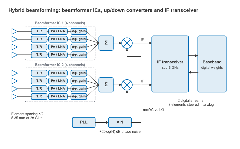
A common building block is a beamformer IC that serves four, eight or sixteen elements. Each channel contains a PA, an LNA, a transmit/receive switch, a phase shifter and a variable-gain stage, and the channels are combined into one RF port through an on-chip splitter/combiner network. Several of these ICs sit under the antenna panel. Their common ports run to an up/down converter, which translates between the millimetre-wave carrier and an intermediate frequency. That IF is often in the sub-6 GHz range, so a transceiver much like those described in Part 12 and Part 13 can handle the final conversion to baseband.

The phase shift can be applied in several places. RF phase shifting places it in the signal path at the carrier frequency and needs only one LO for the whole array, but the phase shifter adds loss ahead of the PA and after the LNA. LO phase shifting moves it into the local-oscillator path, where loss is easier to tolerate, at the cost of distributing an LO to every channel. All of these are phase shifters, not delays, which matters for wideband signals.

Beam squint

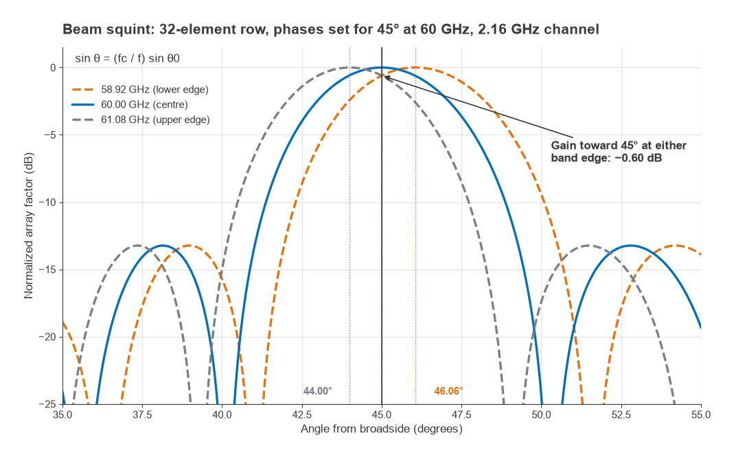
Part 18 introduced beam squint in general terms. At millimetre-wave channel widths it becomes a design constraint. A phase shifter applies a fixed phase across the band, whereas the phase difference that steers a beam to angle θ₀ is proportional to frequency. Phases set correctly at the centre frequency f_c steer a different frequency f toward

sin θ = (f_c/f) sin θ₀

so the beam moves across the band. For a 400 MHz channel at 28 GHz steered to 45°, the band edges at 27.8 and 28.2 GHz point to 45.41° and 44.60°. For an 8-element row with a half-power beamwidth near 18° at that steering angle, the error is invisible. For a 2.16 GHz channel at 60 GHz the edges, 1.08 GHz either side of centre, point to 46.06° and 44.00°. A 32-element row steered to 45° has a beamwidth of about 4.5°, and its gain toward the intended angle falls by 0.60 dB at both band edges. True-time-delay elements remove the effect but are larger and lossier than phase shifters, so designers usually keep sub-arrays small enough that squint stays tolerable and apply true delay, if at all, between sub-arrays.

EIRP, Power and Heat

In a transmitting array the element powers add, and the array gain also rises with element count. For N elements each delivering P_el to an element of gain G_el, with coherent combining in the beam direction,

EIRP = P_el + 10log(N) + 10log(N) + G_el = P_el + 20log(N) + G_el

The first 10log(N) is the total conducted power, the second the array gain, so doubling the element count adds 6 dB of EIRP.

Worked example: EIRP and DC power of a 64-element panel

Take the 8 × 8 panel from the path-loss example, with each channel delivering +10 dBm (10 mW) of average power and an assumed element gain of 5 dBi.

• Total conducted power: 10 + 10log(64) = 10 + 18.06 = 28.06 dBm, or 640 mW.
• EIRP: 10 + 36.12 + 5 = 51.12 dBm.

Achieving 51 dBm EIRP from a single element of 5 dBi would need 46.1 dBm, or about 41 W, from one PA at 28 GHz. Spread across 64 channels the requirement is 10 mW each. The cost appears in DC power. If each PA reaches a power-added efficiency of 15% at its operating back-off, an assumed figure for illustration, it draws 10/0.15 = 66.7 mW, and the 64 PAs together draw 4.27 W to radiate 640 mW. Everything else in the channel comes on top of that. Removing several watts of heat from an area a few centimetres square, directly behind an antenna that cannot be covered by a metal heat sink, is one of the main constraints on millimetre-wave product design.

The receive side scales more gently. Each element contributes uncorrelated noise from its own LNA while the signal adds coherently, so the SNR improves by 10log(N), not 20log(N). The 64-element panel improves receive SNR by 18.06 dB relative to one element, plus the element gain. Per-channel noise figure still matters as much as in Part 4, so each LNA sits as close to its element as the layout allows.

LO Generation and Phase Noise

Synthesizing a clean LO directly at 28 GHz or 60 GHz is difficult. A common approach is to synthesize a lower frequency and multiply it, or to run a VCO at a lower frequency and use frequency multipliers. As described in Part 10, multiplying a signal by N multiplies its phase deviations by N as well, so the phase noise rises by 20log(N). Multiplying a 3.5 GHz synthesizer by 8 to reach 28 GHz raises its phase noise by 18.06 dB. A source with −110 dBc/Hz at 100 kHz offset becomes −91.9 dBc/Hz at the same offset at 28 GHz.

OFDM systems respond to this by spacing subcarriers further apart. 5G NR in FR2 uses subcarrier spacings of 60 kHz and 120 kHz for data, compared with 15 kHz or 30 kHz in most sub-6 GHz deployments. Wider spacing reduces the inter-carrier interference caused by phase noise and tolerates the larger Doppler shifts of a higher carrier. NR additionally defines a phase-tracking reference signal so the receiver can estimate and remove the common phase error symbol by symbol. Phase noise at these frequencies is managed jointly by the synthesizer and the waveform.

LO distribution across a large array adds its own problems. Every channel or sub-array needs an LO with a controlled phase relationship to its neighbours, and phase drift between them appears directly as beam-pointing error and lost gain. Arrays are therefore calibrated, often through built-in loopback paths.

Putting a Millimetre-Wave Radio Together

Gathering the threads, a typical millimetre-wave terminal or small cell has a recognizable structure. An antenna panel with tens to hundreds of elements sits directly on beamformer ICs, one channel per element, each channel with its own PA, LNA, switch and phase control. The beamformer ports combine into a few streams, each converted to and from an IF by a dedicated up/down converter with a multiplied LO. A sub-6 GHz transceiver, or a set of data converters, carries those streams to baseband, where the digital part of the hybrid beamformer and the beam-management algorithms live.

The blocks are the ones this series has covered since Part 1. What differs is the budget: small power per PA but large EIRP, ordinary LNAs sharing one beam, and every figure now a function of beam direction, which makes measurement considerably harder.

Next in the Series

The final part, Part 20, Measuring Radio Performance, turns from design to verification. It covers how noise figure, EVM, adjacent-channel leakage and sensitivity are measured on the bench, how instrument limits and uncertainty enter the result, and how over-the-air methods take over when an array like the one in this part has no connector to measure through.