

Part 17, Antennas and Propagation for Radio Designers, treated the antenna as a single element with a fixed pattern. Its gain came from physical aperture, and pointing it meant turning it. Put several antennas side by side, give each its own amplitude and phase, and the pattern becomes something the radio controls electronically. The same set of antennas can form a narrow beam, steer it in microseconds, place a null on an interferer, or carry several independent data streams through one channel.
This part covers array gain, beam steering, element spacing and the analog, digital and hybrid architectures that implement them, and ends with spatial multiplexing, where multiple antennas are used for capacity rather than gain.
Why Multiple Antennas: Array Gain
Consider N identical elements, each driven by its own power amplifier at power P, with phases set so that the fields add in phase in one direction. In that direction the field amplitude is N times that of one element, so the power density is N2 times larger. Half of that improvement, a factor of N, is simply the extra total power of N amplifiers. The other factor of N is directivity: the array concentrates its radiation into a narrower beam. The EIRP therefore rises as
EIRP = P + Ge + 20log(N)
with P in dBm and Ge the element gain in dBi. On receive the picture differs. Each element collects the signal with its own independent thermal noise. Combining the outputs coherently adds the signals in amplitude and the noise in power, so the SNR improves by 10log(N). A 16-element receive array gains 12 dB of SNR over one element, and a 16-element transmit array gains 24 dB of EIRP for the same per-element PA power.
The 20log(N) law is the main attraction of active arrays at high frequencies. Many small PAs, each well within the capability of a silicon process, combine in space with no combiner loss.
The Array Factor and Beam Steering
For a uniform linear array of N elements spaced d apart, the far-field pattern is the element pattern multiplied by the array factor. With equal amplitudes, the normalized array factor is
AF(θ) = sin(Nψ/2) / (N sin(ψ/2)), with ψ = (2πd/λ)(sinθ − sinθ0)
where θ is measured from broadside and θ0 is the steering angle. The beam is steered by applying a progressive phase shift between adjacent elements of
Δφ = −360° (d/λ) sinθ0
With half-wavelength spacing, steering to 30° needs 360 × 0.5 × sin30° = 90° of phase step between elements. Element 16 is then 15 × 90° = 1350° away from element 1. A phase shifter only needs to cover 0 to 360°, so it applies the same shift modulo 360°.
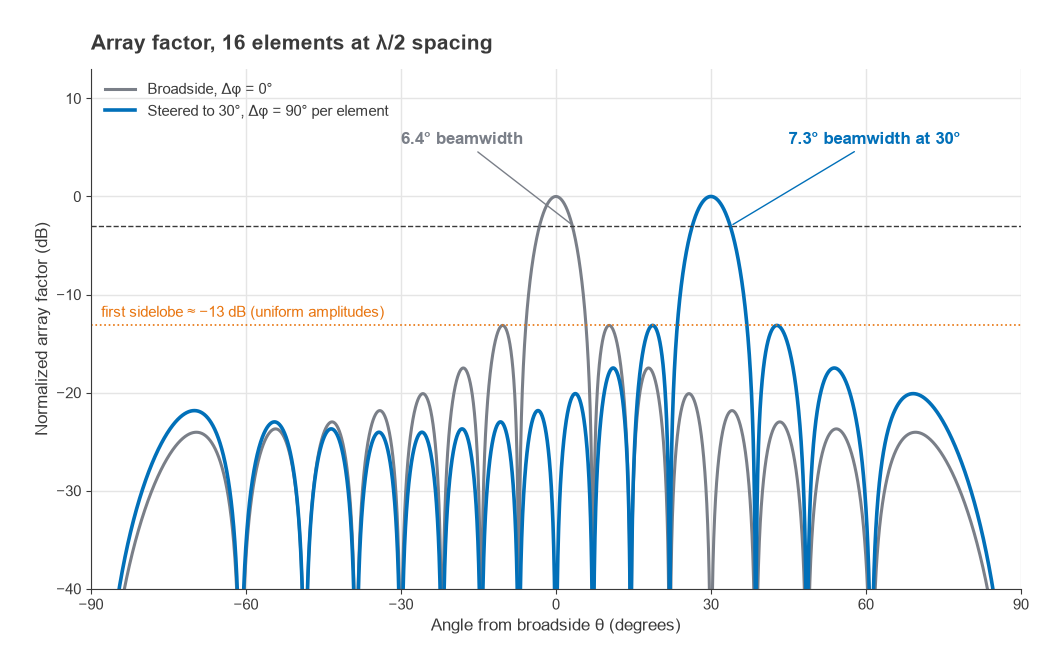
At broadside, the half-power beamwidth of a uniform array is approximately
θ3dB ≈ 0.886 λ/(Nd) radians
For N = 16 and d = λ/2, this gives 0.886 × 2/16 = 0.111 rad, or 6.3°. Evaluating the array factor exactly gives 6.36°. When the beam is steered, the projected length of the array shrinks by cosθ0 and the beam broadens by roughly 1/cosθ0, to 7.3° at 30°. Directivity falls in proportion, and the element pattern, which usually also falls away from broadside, adds to the loss. This scan loss is why planar arrays are rarely asked to cover more than about ±60°.
With uniform amplitudes the first sidelobes sit about 13 dB below the main beam. Tapering the amplitudes towards the array edges, with a Taylor or Chebyshev weighting, lowers the sidelobes at the cost of a wider beam and some loss of gain, the same trade seen with reflector illumination in Part 17. On transmit, a taper means that the edge PAs run below their rated power, so tapering costs EIRP as well as directivity.
Grating Lobes and Element Spacing
The array factor is periodic in ψ. Whenever ψ reaches a multiple of 2π, every element is again in phase and a second main beam, a grating lobe, appears. Grating lobes stay out of visible space provided
d/λ < 1 / (1 + |sinθmax|)
where θmax is the largest steering angle. For a scan range of ±60°, d < 0.536λ. Half-wavelength spacing satisfies this for any scan angle, which is why it is the default.
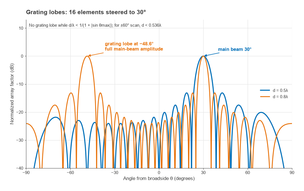
The penalty for wider spacing is severe. An array with d = 0.8λ steered to 30° has a grating lobe where sinθ = 0.5 − 1/0.8 = −0.75, at −48.6°, with the same amplitude as the main beam. Energy radiated there is lost from the link and lands on whatever lies in that direction. On receive, an interferer at −48.6° is received with full array gain.
The spacing rule interacts with packaging. At 3.5 GHz, λ/2 is 43 mm and there is room behind each element for an amplifier, a phase shifter and a filter. At 28 GHz it is 5.4 mm, and the electronics behind each element must fit in that pitch or be moved off to the side through feed lines that add loss. The spacing must also be set at the highest operating frequency, since d/λ grows with frequency.
Analog, Digital and Hybrid Beamforming
There are three basic ways to apply the per-element weights.
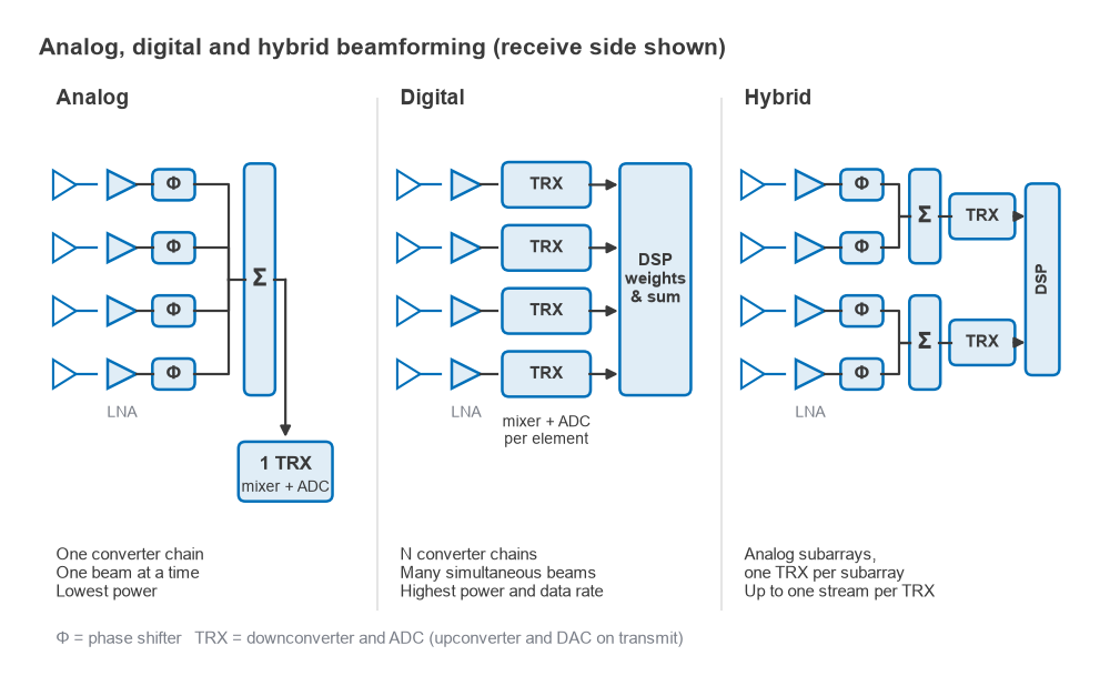
Analog beamforming places a phase shifter, and often a variable-gain amplifier, in each element path at RF or IF, and combines the paths before a single transceiver. Only one data converter pair and one up/down-conversion chain are needed, so power and cost are low. The limitation is that the whole array forms one beam at a time, set by the phase shifters.
Digital beamforming gives every element its own full transceiver: LNA and PA, mixers, synthesizer distribution and converters. The weights are applied as complex multiplications in the digital domain, so any number of simultaneous beams can be formed from the same samples, nulls can be placed precisely, and the weights can vary with frequency across the channel. The cost is N times the converter power and data rate. Part 13 showed how direct RF sampling reduces the analog hardware per channel, but converter power still scales with the number of elements.
Hybrid beamforming divides the array into subarrays. Each subarray is steered by analog phase shifters and feeds one digital transceiver. A 64-element array built as four subarrays of 16 elements needs four transceivers instead of 64 and can form up to four digitally weighted beams or streams. It is the usual compromise at millimetre-wave frequencies, where element counts are high and converter power is significant.
Analog phase shifters introduce two errors that digital weights avoid. The first is quantization. An n-bit phase shifter has a step of 360°/2n, and if the errors across elements are random and uniform, the RMS phase error is the step divided by √12. A 6-bit shifter has a step of 5.625° and an RMS error of 1.62°, or 0.028 rad. The resulting gain loss, about 10log(e−σ²), is only 0.003 dB, and with 4 bits it is still only 0.06 dB. The larger effect of coarse quantization is on sidelobes, since correlated rounding errors along the array produce quantization lobes.
The second error is beam squint. A phase shifter provides a fixed phase, which equals the required time delay at only one frequency. At other frequencies the beam points to
sinθ = sinθ0 (f0/f)
Steered to 45° at f0, the beam points to 42.3° at 1.05f0 and 48.1° at 0.95f0. For a 16-element array, whose beamwidth at 45° is about 9.0°, that is almost a third of a beamwidth at each edge of a 10% band, and the edge of the channel sees reduced gain. True-time-delay elements, or digital beamforming with frequency-dependent weights, remove squint. They become necessary when the fractional bandwidth or the array size is large.
All three architectures need calibration. Each element path has its own gain and phase tolerances, which drift with temperature and differ between PAs. Arrays include coupling paths or reference receivers so that these errors can be measured and corrected in operation.
Worked Example: A 64-Element Transmit Array
An 8 × 8 planar array with half-wavelength spacing drives each element with a PA delivering +10 dBm (10 mW). An element in such an array occupies an area of (λ/2)2, so its effective gain is 4π(λ2/4)/λ2 = π, or 4.97 dBi, assuming no loss.
- Total conducted power: 64 × 10 mW = 640 mW, or 10 + 18.06 = +28.06 dBm.
- Array directivity: 4.97 + 18.06 = 23.03 dBi, which matches 4π(64 × λ2/4)/λ2 = 64π.
- EIRP at broadside: 10 + 4.97 + 20log(64) = 10 + 4.97 + 36.12 = +51.1 dBm.
- Beamwidth in each plane: 0.886 × 2/8 = 0.22 rad, or about 12.7°.
To reach the same EIRP from a single element with 4.97 dBi of gain, one PA would have to deliver +46.1 dBm, about 41 W. The array gets there with 64 amplifiers of 10 mW each. That comparison explains why phased arrays dominate at millimetre-wave frequencies, where a single 41 W PA is impractical and feed losses would be prohibitive.
Used as a receiver, the same array improves SNR by 18.06 dB over one element. In a link budget like that of Part 15, that is equivalent to replacing a 5 dBi receive antenna with a 23 dBi one, with the difference that the beam can be pointed electronically and can follow a moving terminal. With a 12.7° beam, pointing accuracy matters: a 6° error puts the far end close to the half-power point.
MIMO and Spatial Multiplexing
Beamforming uses multiple antennas to send one stream with more gain. Spatial multiplexing uses them to send several streams at once over the same frequency. If a channel has Nt transmit and Nr receive antennas and enough scattering that the paths between them are sufficiently different, the receiver can separate up to min(Nt, Nr) independent streams.
For a single antenna pair in AWGN, the Shannon capacity is C = B log2(1 + SNR). At 20 MHz and 20 dB SNR this is 20 × log2(101) = 133 Mb/s. For a MIMO channel with matrix H and total transmit power split equally across the transmit antennas, the capacity becomes
C = B log2 det(I + (SNR/Nt) HHH)
A Monte Carlo evaluation over independent Rayleigh-fading channels at 20 dB average SNR gives mean spectral efficiencies of about 5.9 b/s/Hz for a single antenna pair, 11.3 b/s/Hz for 2 × 2 and 22.1 b/s/Hz for 4 × 4. In a 20 MHz channel that is roughly 118, 226 and 443 Mb/s. Capacity grows almost linearly with the number of antennas at the same total power and bandwidth, which no other technique offers.
Those figures assume uncorrelated paths. A line-of-sight channel between closely spaced arrays has nearly identical paths and supports far fewer streams, which is why dual polarization is used to obtain at least two streams even in line of sight. The radio hardware also has to keep the streams distinct. Each stream needs its own transceiver chain, LO phase noise must be common or well controlled across chains, and coupling between antennas or chains mixes the streams before the receiver can separate them. The EVM of each chain from Part 16 now sets the ceiling on how many high-order streams can be decoded at once.
Next in the Series
Phased arrays, high element counts and tight element pitch all come together at millimetre-wave frequencies. Part 19, Millimeter-Wave Radio Architectures, looks at what changes above about 24 GHz: path loss and atmospheric absorption, the packaging of antennas with the electronics, the power and heat budget behind the required EIRP, and the LO phase noise that limits high-order modulation.