


RF fundamentals are the small set of ideas behind every radio: frequency and wavelength, power in dBm, impedance and reflection, resonance, path loss, noise and modulation. This guide to RF engineering fundamentals works through each one with real figures, using a single 915 MHz link from transmitter to receiver.
Radio frequency usually means signals from a few kilohertz to around 300 GHz. For a topic-by-topic index with detailed pages on decibels, Q factor and skin depth, use the RF fundamentals hub. For a study plan, see the RF engineer roadmap. Here the aim is narrower: to show how the core concepts connect, by carrying one set of numbers all the way through.
RF Basics Through One Worked Link
The example is a low-data-rate link with these assumptions:
- Frequency 915 MHz, transmit power +20 dBm
- Antenna gain 2.15 dBi at each end, spacing 500 m
- Receiver bandwidth 125 kHz, noise figure 6 dB, required SNR 10 dB
- Transmit antenna impedance 75 + j25 Ω on a 50 Ω system
The values are illustrative. They were chosen because they are close to what a small sensor radio might use, and each section below takes one step of the calculation.
Frequency and Wavelength
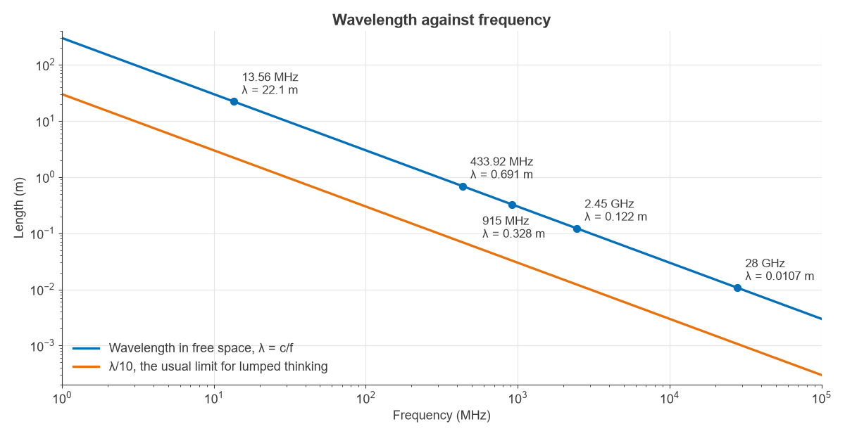
Wavelength is λ = c/f, where c is about 2.998 × 10⁸ m/s. At 915 MHz that gives λ = 0.328 m, and one cycle lasts 1.09 ns. A quarter-wave antenna is 81.9 mm long, and λ/10 is 32.8 mm.
The λ/10 figure matters because it is the usual limit for treating a conductor as a plain wire. A longer connection carries a visibly different phase at each end, so it has to be analysed as a transmission line. That one idea separates RF theory from low-frequency circuit theory. The RF frequency bands page shows how the spectrum is divided.
Power in dBm
RF power spans too wide a range for watts to be convenient, so engineers use dBm, which is power relative to 1 mW on a logarithmic scale. Our +20 dBm transmitter puts out 100 mW.
Power and voltage are tied together by the system impedance. In 50 Ω, 100 mW is:
- 2.24 V RMS and 44.7 mA RMS
- 3.16 V peak, or 6.32 V peak to peak
The peak figure is useful when checking whether a signal will overdrive a part. Gains and losses in decibels simply add, which is why the link budget later in this example is plain addition. The full method is on the dB and dBm page, and average and peak power are defined in power in RF systems.
Impedance and Reflection
Maximum power reaches a load when it is matched to the source. Most RF systems use 50 Ω, so any other load reflects part of the incident wave. The reflection coefficient is:
Γ = (ZL − Z0) / (ZL + Z0)
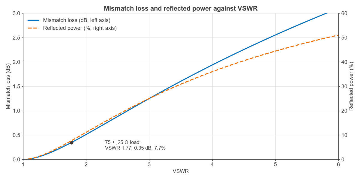
For the antenna at 75 + j25 Ω, |Γ| = 0.277 at an angle of 33.7°. From that magnitude:
- VSWR = (1 + |Γ|) / (1 − |Γ|) = 1.77
- Return loss = −20 log10|Γ| = 11.1 dB
- Reflected power = |Γ|2 = 7.7%
- Mismatch loss = −10 log10(1 − |Γ|2) = 0.35 dB
So 92.3 mW of the 100 mW reaches the antenna, or +19.65 dBm. A mismatch of this size costs little power, as Figure 2 shows. It starts to matter when a filter or an amplifier sits on either side, because both are designed around a 50 Ω load. See VSWR and return loss and L-network matching for how to correct it.
Resonance and Q
An inductor and a capacitor store energy in different forms and exchange it at the resonant frequency f0 = 1/(2π√(LC)). Radios use resonance to pick out one frequency, in filters, matching networks and oscillators.
Take 10 nH and 3 pF. They resonate at 918.9 MHz, close to our operating frequency. The reactance of each part there is 57.7 Ω. With 2 Ω of series resistance, Q = X/R = 28.9, and the 3 dB bandwidth is f0/Q = 31.8 MHz. Higher Q gives a narrower filter and lower loss, but component tolerance then matters more. A real part also has parasitics that shift these values, as explained on the Q factor and component parasitics pages.
Path Loss and Propagation
A radio wave spreads out as it travels. Free-space path loss describes that spreading between two isotropic antennas:
FSPL = 20 log10(4πd/λ)
At 500 m and 915 MHz, FSPL = 85.66 dB. Adding up the link:
| Item | Value |
|---|---|
| Transmit power | +20.00 dBm |
| Mismatch loss | −0.35 dB |
| Transmit antenna | +2.15 dBi |
| Receive antenna | +2.15 dBi |
| Path loss | −85.66 dB |
| Received power | −61.70 dBm |
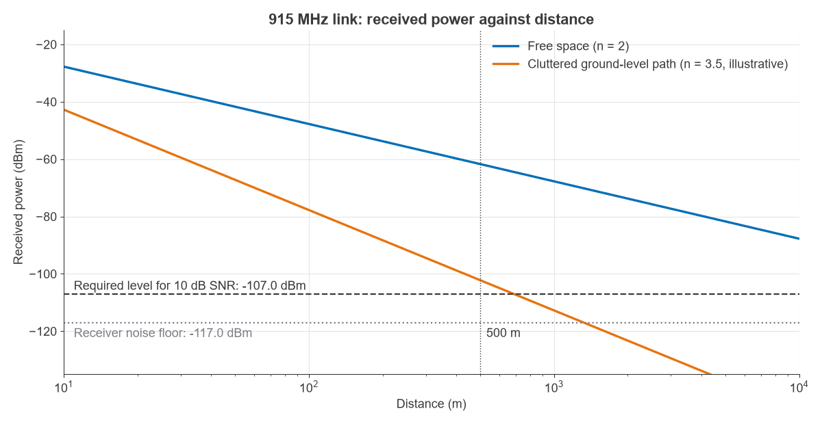
That is 0.68 nW, about 148 million times less than the 100 mW sent, or 81.7 dB. Real paths lose more. A common empirical model replaces the factor of 20 with 10n, where n is the path loss exponent, starting from the free-space loss at 1 m. With n = 3.5 for a cluttered path at ground level, the loss at 500 m becomes 126.1 dB and received power falls to −102.2 dBm. The RF link budget page extends this method, and antennas covers the gain terms.
Noise and Sensitivity
Every receiver has a noise floor set by thermal noise, kTB, which is −174 dBm/Hz at room temperature. In a 125 kHz bandwidth that gives −123.0 dBm. The receiver adds its own noise, described by a noise figure of 6 dB, so the effective floor is −117.0 dBm.
The signal-to-noise ratio is then the received power minus that floor:
- Free space: −61.70 − (−117.03) = 55.3 dB
- Cluttered path: −102.19 − (−117.03) = 14.8 dB
The receiver needs 10 dB, which puts its sensitivity at −107.0 dBm. The cluttered path has only 4.8 dB of margin, and it runs out at about 690 m. That one number, the margin, is what most of RF engineering works to protect. See thermal noise and kTB for the derivation, and the RF noise section for more.
Modulation and Bandwidth
A carrier carries no information until something varies it. Amplitude modulation changes its size, frequency modulation its frequency and phase modulation its phase. Digital schemes such as QPSK and QAM switch between defined amplitude and phase states.
The Shannon limit, C = B log2(1 + SNR), sets the ceiling for a channel. In 125 kHz, an SNR of 14.8 dB allows about 622 kbit/s and an SNR of 55.3 dB allows about 2.30 Mbit/s. Real modems stay below these limits. Bandwidth and SNR trade against each other, so a narrower channel lowers the noise floor at the cost of data rate. The modulation, EVM and PAPR part of the radio architectures series covers this in depth.
How the RF Fundamentals Connect
The worked example shows that the core concepts are one calculation seen from different points. Wavelength sets the antenna size and the path loss. Impedance decides how much power gets into the antenna. Resonance selects the channel. Noise and bandwidth set what the receiver can recover, and modulation decides how much data that SNR will carry.
To apply these ideas to hardware, the RF circuit design basics article works through a first stage in detail.
Frequently Asked Questions
What is RF in engineering?
RF stands for radio frequency. In engineering it refers to electrical signals and electromagnetic waves used for wireless communication, radar, sensing and heating, roughly from kilohertz up to 300 GHz. RF engineering is the design and testing of the circuits and systems that handle them.
What are the basics of RF theory?
The main topics are wavelength, decibels, impedance and reflection, resonance, path loss, noise and modulation. Maxwell’s equations sit underneath all of them, but a beginner can use the results above without deriving them first.
Why do RF engineers use 50 ohms?
Fifty ohms is a long-standing compromise for coaxial cable, sitting between the impedance for lowest loss, about 77 Ω, and the impedance for highest power handling, about 30 Ω. Using one standard value lets parts from different sources connect without reflections.
What is the best way to learn RF for beginners?
Work through the calculations by hand, then check them in simulation or on a bench. The learn RF design page gives a full curriculum.
Related Topics
Continue with the RF fundamentals hub, the RF design guide and the RF calculators. To see how these skills are used at work, read what an RF engineer does.