Antenna Matching and Tuning in Products

Antenna matching is the process of measuring an antenna’s input impedance in its final product environment and adding a small reactive network, usually a pi footprint of chip inductors and capacitors, so that the antenna presents close to 50 Ω to the radio across the operating band. The work is done with a calibrated vector network analyzer connected at the antenna feed, with the enclosure, battery and nearby parts in place, because those parts shift the antenna’s resonance and impedance.

This page sets out the procedure engineers follow on real products: why the match must be done in the enclosure, how to set up the measurement, how to choose pi-network values from a Smith chart, and what a match can and cannot recover. A worked 2.45 GHz example runs through the whole process. The page belongs to the antennas hub within the wider RF design reference, and it builds on general impedance matching theory.

Why antennas need matching in the product

A printed or chip antenna is usually designed on a bare evaluation board. In the product, plastic housings add dielectric loading that lowers its resonant frequency, batteries, displays and shield cans couple to its near field, and the ground plane, which carries much of the radiating current for small antennas such as the inverted-F, may differ in size. Each effect moves the impedance seen at the feed.

The result is that an antenna that showed a good return loss on its own board can show 5 dB or less in the finished product. The fraction of power reflected back to the radio is |Γ|², and the corresponding mismatch loss is:

ML = −10 log₁₀(1 − |Γ|²) dB

A return loss of 5 dB corresponds to |Γ| ≈ 0.56 and a mismatch loss of about 1.6 dB in both transmit and receive. Over a link, that loss reduces range in the same way as a weaker antenna. The relationships between Γ, VSWR, return loss and mismatch loss are tabulated on the VSWR and return loss page.

Planning the pi-network footprint

Because the final impedance is unknown at layout time, the usual practice is to place a three-element pi footprint (shunt, series, shunt) between the radio’s 50 Ω line and the antenna feed. Fitting a 0 Ω resistor in the series position and leaving both shunt positions empty gives a straight-through connection, so the board works before any tuning. After measurement, any two of the three positions can implement an L-network, and all three give a pi network when more bandwidth control is needed.

• Place the footprint close to the antenna feed, so the line between the network and the antenna is short and its transformation is small.
• Use pad sizes for the smallest practical part (often 0402 or 0201) to keep pad capacitance low.
• Give each shunt pad its own ground via, placed right at the pad, as described in RF grounding and via stitching.
• Keep the feed line a controlled 50 Ω trace, sized with the microstrip calculator or as grounded coplanar waveguide.

The pi footprint gives full coverage of the Smith chart. A two-element L-network can match any load with a positive real part, provided the right topology is chosen, and the theory behind each topology is on the L-network matching and pi and T matching networks pages.

Measuring the antenna impedance in the enclosure

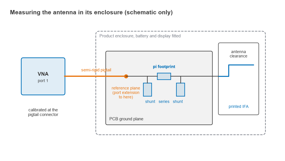
The measurement must reproduce the conditions the antenna will see in use, and it must place the VNA’s reference plane at the input of the pi network. A common setup is a short semi-rigid coaxial pigtail soldered to the board, with its centre conductor on the feed trace and its shield bonded to ground at several points.

Step-by-step measurement procedure

1. Disconnect the radio output from the feed line, typically by removing a 0 Ω link, so that the radio does not load the measurement.
2. Solder the pigtail at the radio side of the pi footprint and route its cable away from the antenna, perpendicular to it where possible.
3. Perform a one-port calibration (open, short, load) at the end of the VNA test cable, then apply port extension or de-embedding to move the reference plane to the pigtail tip. VNA calibration and de-embedding cover both steps.
4. Verify the reference plane: with the series position open, the trace should sit near the open point of the Smith chart; with it shorted to ground, near the short point.
5. Assemble the full product: housing closed, battery, display and cables in place, and the device in its normal orientation.
6. Record S11 across the band and a margin either side, and save it as a Touchstone file for use in a circuit simulator.

The pigtail cable itself is a source of error. Current on the outside of the shield makes the cable part of the antenna, so the reading changes when the cable moves. Ferrite sleeves near the board reduce this; if moving the cable during a live sweep shifts the trace, fix the shield currents before choosing any values.

Repeat the measurement for each use condition that matters, such as on a table, in a hand or on a metal surface. Tissue and metal both detune the antenna, so the final match is usually a compromise across these cases. Basic VNA operation is described on the VNA basics page.

Worked example: matching a 2.45 GHz antenna

Suppose the in-enclosure measurement of a printed inverted-F antenna gives Z_A = 20 − j30 Ω at 2.45 GHz. The antenna resonates above the band, so it looks capacitive at the band centre. The reflection coefficient is:

Γ = (Z_A − 50)/(Z_A + 50) = (−30 − j30)/(70 − j30), so |Γ| = 0.557

That is a return loss of 5.1 dB and a mismatch loss of 1.61 dB. Only 69% of the available power reaches the antenna.

Choosing the network on the Smith chart

Since R_A = 20 Ω is below 50 Ω, the first element from the antenna side is a series reactance that moves the load onto the g = 1 circle, the set of impedances whose admittance has a real part of 1/50 S. The condition is:

R/(R² + X²) = 1/Z₀, which gives X = ±√(Z₀R − R²) = ±√(1000 − 400) = ±24.5 Ω

Two solutions follow. To reach X = +24.5 Ω from −30 Ω, the series element must add +54.5 Ω, an inductor of 54.5/(2π × 2.45 GHz) = 3.54 nH. The admittance is then 0.020 − j0.0245 S, and a shunt capacitor with susceptance +0.0245 S cancels the imaginary part: C = 0.0245/ω = 1.59 pF. The alternative path to X = −24.5 Ω needs a series capacitor of 11.8 pF followed by a shunt inductor of 2.65 nH.

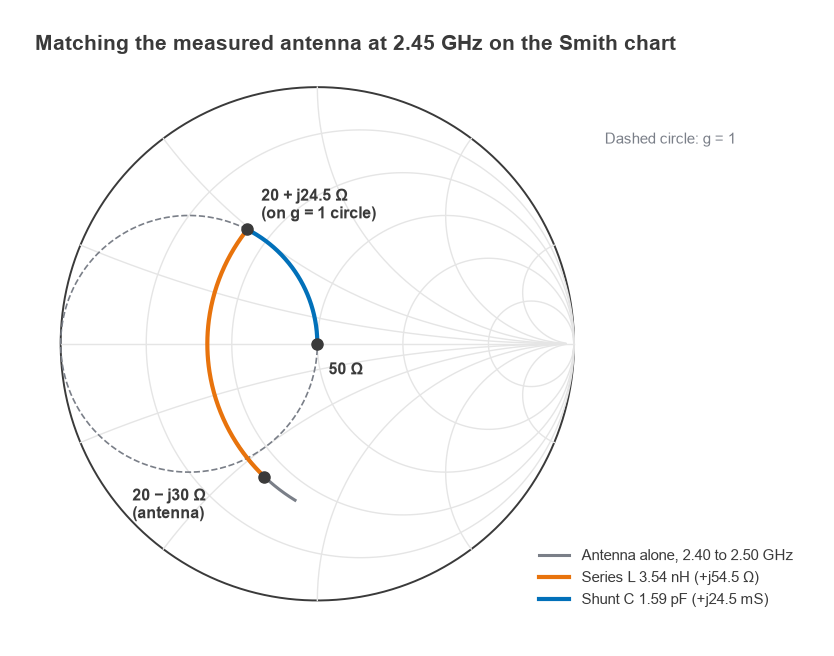
The first solution is a low-pass network, which helps attenuate transmitter harmonics, and its values are convenient. In the pi footprint, the 3.6 nH series inductor (nearest standard value) goes in the series position and the 1.6 pF capacitor goes in the shunt position on the radio side. The antenna-side shunt position stays empty. Rounding to standard values still gives a computed return loss of 32 dB at 2.45 GHz with ideal parts.

Component losses and bandwidth

Real chip parts have finite Q. Taking an inductor Q of 40 and a capacitor Q of 200 at 2.45 GHz, values of the order quoted for small chip parts at this frequency, the computed return loss at the centre is 27.5 dB. Of 1 W available from the radio, 0.928 W reaches the antenna, a total loss of 0.33 dB, almost all of it dissipated in the inductor. Compared with the 1.61 dB lost to mismatch before matching, the net improvement is about 1.3 dB.

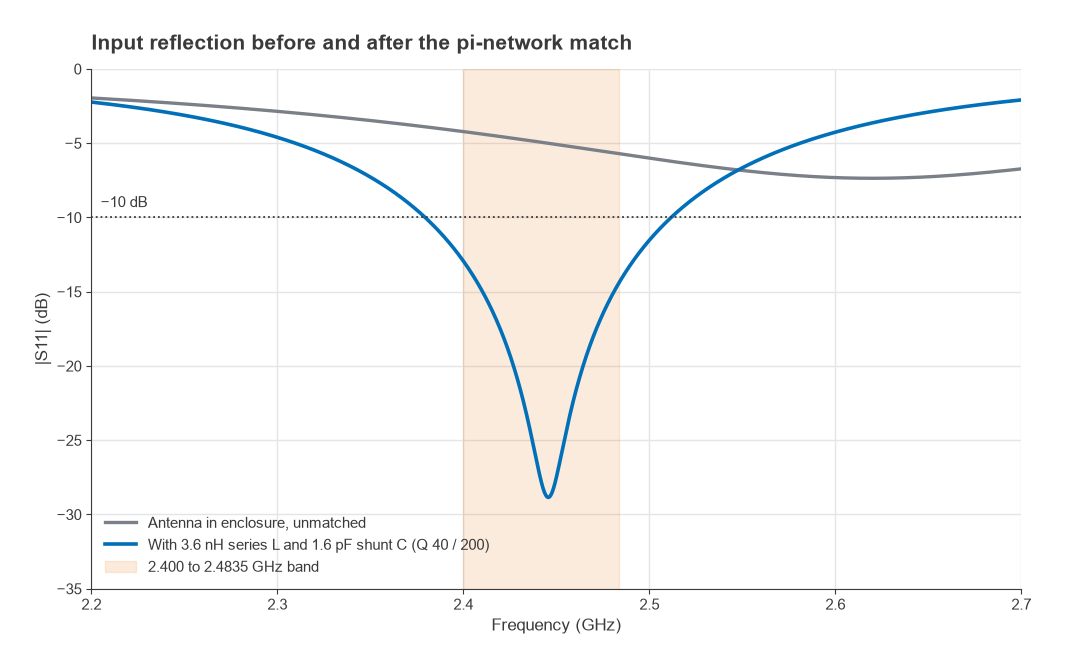
Using a simple series-RLC model of the antenna fitted to the measured point (resonance near 2.62 GHz, antenna Q about 11), the matched −10 dB bandwidth runs from 2.380 to 2.512 GHz. Return loss is 12.9 dB at 2.400 GHz and 14.4 dB at 2.4835 GHz, so the whole 2.4 GHz ISM band clears the usual 10 dB target. In practice, the measured Touchstone file replaces the model, and the simulator sweeps the actual standard values to confirm the band edges.

Quantity at 2.45 GHz	Unmatched	Matched (3.6 nH, 1.6 pF)
Impedance seen by radio	20 − j30 Ω	50.9 − j4.2 Ω
Return loss	5.1 dB	27.5 dB
Power reaching antenna	69%	92.8%
Total loss before antenna	1.61 dB	0.33 dB
−10 dB bandwidth	none	2.380 to 2.512 GHz

Practical tuning in the lab

Calculated values are a starting point, since pad parasitics and part variation shift the result. A practical loop:

1. Load the measured S11 into a circuit simulator and model each pad as a small shunt capacitance if its value is known.
2. Use vendor S-parameter models of the candidate chip parts rather than ideal L and C, since they include self-resonance and loss. See RF component parasitics.
3. Fit the parts, close the enclosure and remeasure. Adjust one value by one standard step at a time and watch which way the trace moves.
4. Centre the match on the band rather than chasing the deepest notch. A broad −12 dB response across the band is more useful than −30 dB at one frequency.
5. Check the result with the other use conditions (hand, table, body) and with production tolerances on part values.

If the resonance is far from the band, matching alone gives a narrow response and more component loss; trimming the antenna element first is better. The PCB antenna design page covers the geometry adjustments.

Multi-band and tunable matching

Antennas that serve two bands, such as 2.4 GHz and 5 GHz Wi-Fi, need an acceptable match at both. A fully populated pi network gives the extra degree of freedom, and a simulator optimiser finds the values. Multi-band cellular devices often use aperture tuners or switched matching networks set by the radio for each band, whose switch losses enter the design budget, as discussed in RF front-end modules.

What matching cannot fix

A good return loss means power reaches the antenna terminals, not that it is radiated. If a battery or metal frame absorbs the near field, or the ground plane is too small, radiation efficiency stays low however good the match. A lossy load near 50 Ω can show an excellent S11 while radiating almost nothing. The antenna parameters page explains how radiation efficiency and mismatch combine into total efficiency.

Matching is therefore followed by radiated measurements: total radiated power (TRP) and total isotropic sensitivity (TIS) in a chamber, or at least a comparative over-the-air test against a reference device. The broader test chain is covered in measuring radio performance, and the system context in antennas and propagation in radio design.

Frequently asked questions

How do you match an antenna?

Measure the antenna’s S11 with a calibrated VNA at the feed point, with the product fully assembled. Plot the impedance on a Smith chart, then choose two or three reactive elements that move it to 50 Ω at the band centre. Fit those parts in a pi footprint, remeasure, and adjust until the band meets the return loss target in every use condition.

What return loss is good enough for a product antenna?

Compact product antennas are commonly tuned for 10 dB of return loss or better across the band, which corresponds to a mismatch loss of about 0.46 dB. Going much further gives little extra radiated power and often narrows the bandwidth.

Why use a pi footprint instead of an L footprint?

The final impedance is unknown when the board is laid out, and different L-network topologies need the shunt element on different sides. A pi footprint covers every case with a single layout, and its third element can trade bandwidth or reach a dual-band compromise.

Related topics

Matching theory is developed in L-network matching, pi and T networks and the Smith chart guide, and values can be checked with the impedance matching calculator. On the antenna side, see PCB antenna design, patch antenna design and antenna parameters. Short definitions of the terms used here are in the wireless terms glossary.