

De-embedding is a post-measurement correction that mathematically removes the known response of test fixtures, launches and lead-in traces from measured S-parameters, leaving the response of the device alone. It works by representing each section as a cascadable matrix and multiplying the measurement by the inverses of the fixture matrices.
A vector network analyzer measures whatever sits between its calibrated ports. When the device under test (DUT) is a surface-mount part on a test board, that includes connectors, launches and lengths of transmission line. This page, part of the S-parameters section of the RF design guide, shows how T-matrix inversion removes them, how the 2x-thru and TRL methods obtain the fixture data, and where the methods go wrong.
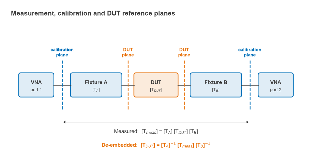
Calibration planes and DUT planes
VNA calibration places the reference plane where the calibration standards connect, usually at the coaxial cable ends. Everything beyond that plane is treated as part of the device. If the DUT sits on a fixture, the measured data describe fixture A, the DUT and fixture B in cascade. Two routes move the reference to the DUT pins:
- Calibrate at the DUT plane with standards built on the fixture itself, as in TRL. The correction happens inside the analyzer.
- Calibrate at the connectors, then de-embed using a model or measurement of each fixture half. The correction happens afterwards, in software.
Both reach the same result when the fixture data are accurate. De-embedding is more flexible: the same measurement can be reprocessed with a better fixture model later, and simulated fixture data from an EM simulation can be used where no physical standards exist.
T-matrix cascade inversion
S-parameters do not cascade by matrix multiplication, because each port’s incident and reflected waves are mixed on both sides of the matrix. Transfer (T) parameters rearrange the waves so that the quantities at port 1 are expressed in terms of those at port 2:
[b1; a1] = [T] · [a2; b2]
With this convention the conversion from S-parameters is
T11 = −ΔS / S21, T12 = S11 / S21, T21 = −S22 / S21, T22 = 1 / S21
where ΔS = S11S22 − S12S21. The inverse conversion is S11 = T12/T22, S21 = 1/T22, S22 = −T21/T22 and S12 = det(T)/T22. Cascaded two-ports now multiply in order, and the DUT follows by inversion:
[Tmeas] = [TA] [TDUT] [TB] ⇒ [TDUT] = [TA]−1 [Tmeas] [TB]−1
The calculation is repeated at every frequency point. Fixture B is usually fixture A with its ports reversed, which in S-parameters means swapping S11 with S22. The T-matrix exists only where S21 ≠ 0, which is no restriction for a fixture but is a reason not to convert a highly isolating DUT on its own. In scikit-rf the whole operation is one line using the network inverse and cascade operators, and fixture data are normally exchanged as Touchstone .s2p files.
Worked example: removing two 20 mm fixture halves at 5 GHz
Each fixture half is modelled as a 0.15 pF launch capacitance at the connector followed by 20 mm of 55 Ω line with an effective permittivity of 3.3 and a loss of 5 dB/m at 1 GHz, scaling with √f. The DUT is a small low-pass T-section: 2 nH series, 0.8 pF shunt, 2 nH series. All values were computed in Python with 50 Ω reference impedance.
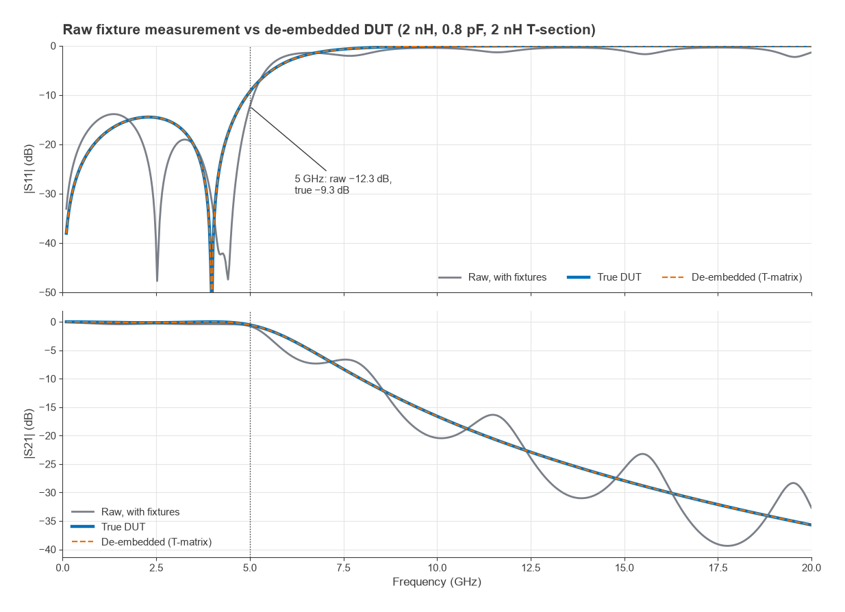
| Quantity at 5 GHz | |S11| | |S21| | ∠S21 |
|---|---|---|---|
| Fixture half A | −21.0 dB | −0.26 dB | 134.7° |
| Raw measurement (A + DUT + B) | −12.3 dB | −0.77 dB | 144.2° |
| De-embedded DUT | −9.3 dB | −0.54 dB | −123.0° |
| True DUT | −9.3 dB | −0.54 dB | −123.0° |
Three points stand out. The raw data make the DUT look better matched than it is, −12.3 dB against −9.3 dB, because the fixture reflections partly cancel the DUT reflection at this frequency. At other frequencies they add instead, which produces the ripple seen in the raw curves. The fixtures add 0.23 dB of loss and about 270° of phase. With an exact fixture model the de-embedded result matches the true DUT to within numerical rounding (a residual of about 10−16), so any error in practice comes from the fixture data, not the algebra.
Getting the fixture data
The inversion needs [TA] and [TB]. There are three common sources:
- Simulation. A 3D EM model of the connector, launch and line. Accuracy depends on how well the model matches the built board, including etch tolerance and dielectric properties.
- 2x-thru measurement. A test coupon with the two fixture halves joined directly, measured and then split into halves.
- On-fixture calibration. TRL or a related method that determines the error terms at the DUT plane directly.
The 2x-thru method
The 2x-thru is the fixture with the DUT removed and the two halves joined, so its length is twice the lead-in length. If the halves are mirror images, the 2x-thru is A cascaded with A reversed. That gives two independent complex equations (S11 and S21 of the 2x-thru) but three unknowns for the half (S11, S22 and S21), so an extra assumption is always needed.
The simplest assumption is that each half is itself symmetric, S11 = S22 = Γ. Solving the cascade then gives a closed form:
Γ = S11,2x / (1 + S21,2x), S21,half = √(S21,2x · (1 − Γ2))
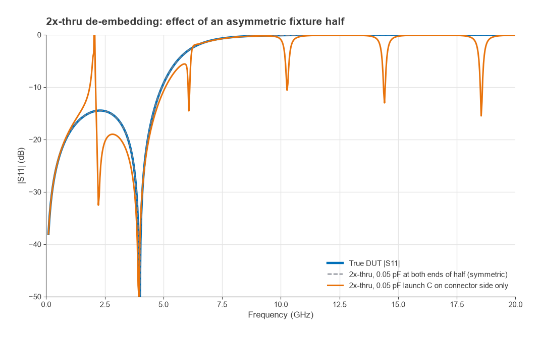
Two practical issues follow directly from the formula. The square root has two signs, so the phase of S21,half must be unwrapped across frequency starting from DC, where it is near zero. And the denominator 1 + S21,2x approaches zero whenever the 2x-thru phase passes through 180°, which makes the extraction sensitive to any measurement error or model mismatch there. For the 40 mm 2x-thru of the example, the phase reaches 180° at about 2.06 GHz.
Real launches are not symmetric. A connector-side launch capacitance with nothing equivalent at the DUT end breaks the assumption. Repeating the worked example with a 0.05 pF launch at the connector side only, the symmetric-half extraction returns |S11| = −10.8 dB at 5 GHz against a true −9.3 dB, and S21 of −0.38 dB against −0.54 dB. Near each 180° crossing of the 2x-thru phase the error becomes large and the de-embedded S11 can exceed 0 dB, which is a clear sign of a bad fixture model. Production 2x-thru algorithms, including those described in the IEEE 370 standard for printed circuit board interconnect characterization, use time-domain and impedance-correction steps to handle asymmetry, and that standard also defines quality checks for the resulting data.
TRL calibration on the fixture
TRL (thru, reflect, line) uses three standards built in the same fixture technology as the DUT: a zero-length or short thru, an identical high reflection (open or short) at each port whose exact value need not be known, and a line longer than the thru. The line’s characteristic impedance sets the reference impedance of the corrected data. TRL solves for the error terms at the DUT plane, so the fixture is removed during calibration rather than afterwards. The method is described further in the VNA calibration article.
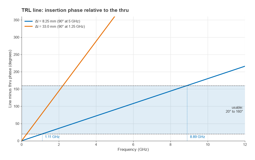
The line standard limits bandwidth. The solution becomes ill-conditioned when the line and thru differ by a multiple of 180°, and a common guideline keeps the difference between about 20° and 160°. For an insertion-phase difference of 90° at the centre frequency f0, the extra length is a quarter of the guided wavelength:
Δl = λg / 4 = c / (4 f0 √εeff)
On a microstrip with εeff = 3.3 and f0 = 5 GHz, λg = 33.0 mm and Δl = 8.25 mm. The phase is 20° at 1.11 GHz and 160° at 8.89 GHz, an 8:1 span. A 33.0 mm line covers 0.28 to 2.22 GHz. Wider ranges use several lines (multiline TRL), and the lowest frequencies are usually handled by a different standard because the line would become impractically long.
| Method | Fixture data from | Main assumption | Typical use |
|---|---|---|---|
| Model-based de-embedding | EM or circuit simulation | Model matches the built fixture | Early work, no test coupons |
| 2x-thru de-embedding | Measured 2x-thru coupon | Halves are mirror images; symmetry or impedance profile known | PCB interconnect and connector characterization |
| TRL calibration | Thru, reflect and line on the fixture | Standards are identical except for line length; line impedance is known | Fixtures, on-wafer, planar devices |
How to de-embed a fixture: step by step
- Design the fixture with matched, identical lead-ins on both sides of the DUT, and put a 2x-thru or TRL coupon on the same panel so it shares the same material and etch.
- Calibrate the analyzer at the coaxial reference plane over the full frequency range, with the same point spacing and IF bandwidth you will use for the DUT.
- Measure the 2x-thru (or build the fixture model) and the DUT on the fixture, and save both as Touchstone files.
- Extract fixture half A and form fixture B by reversing its ports.
- Convert all data to T-parameters, compute [TA]−1[Tmeas][TB]−1 at each frequency and convert back to S-parameters.
- Check the result: de-embedding the 2x-thru itself should give a near-ideal zero-length thru, a passive DUT must have |S11|2 + |S21|2 ≤ 1, and the impulse response should be causal.
Lossy fixtures amplify noise. Removing 10 dB of fixture loss also multiplies the trace noise on S21 by about 10 dB, so keep lead-ins short and use a narrower IF bandwidth or averaging when the fixture is long. For differential DUTs the same process applies to four-port data before conversion to mixed-mode S-parameters, and the lead-ins are usually grounded coplanar waveguide for a clean launch.
Frequently asked questions
What is de-embedding?
De-embedding is the removal of a known fixture’s effect from measured S-parameters. The fixture halves and the measurement are converted to T-parameters, and the measurement is multiplied by the inverse fixture matrices on each side. The result is the response at the DUT pins rather than at the coaxial connectors.
What is the difference between calibration and de-embedding?
Calibration measures known standards to correct the analyzer’s systematic errors up to a reference plane. De-embedding removes a known network beyond that plane after the measurement. TRL on a fixture combines both by placing the calibration plane directly at the DUT.
What is a 2x-thru?
A 2x-thru is a fixture coupon with the two lead-in halves joined directly, without the DUT. Measuring it gives the combined response of both halves, which is then split into a single-half model. Splitting needs an assumption about symmetry or impedance, and the accuracy of the de-embedded data depends on it.
Why does my de-embedded S11 go above 0 dB?
A passive device cannot reflect more power than it receives, so |S11| above 0 dB means the fixture model does not match the real fixture. Common causes are asymmetric launches, a 2x-thru extraction near a 180° phase crossing, or a coupon whose lead-ins differ from those on the DUT board.
Related topics
The instrument side is covered in VNA basics and VNA calibration. Corrected two-port data feed directly into power gain definitions and stability analysis, and can be viewed on a Smith chart. All of these belong to the S-parameters hub.