Antenna Parameters: Gain, Directivity, Efficiency, Beamwidth

Antenna gain is the ratio of the power density an antenna radiates in its strongest direction to the power density an ideal lossless isotropic radiator would produce with the same input power, usually quoted in dBi. It equals directivity multiplied by radiation efficiency, so it describes both how tightly the antenna focuses energy and how much of that energy survives conductor and dielectric loss.

Gain is one of a small set of antenna parameters that together describe what an antenna does to a signal: directivity, efficiency, radiation pattern, beamwidth, sidelobe level, polarization and impedance bandwidth. These figures feed straight into a link budget, set the EIRP of a transmitter, and decide how much interference a receiver collects from off-axis sources. This page defines each one, shows how they relate, and works through a realistic example. It sits under the antennas hub of the wider RF design reference.

Directivity: how an antenna concentrates power

Every real antenna radiates more in some directions than others. The radiation intensity U(θ, φ) is the power radiated per unit solid angle, in watts per steradian. An isotropic radiator spreads its total radiated power P_rad evenly over 4π steradians, so its intensity is P_rad/4π everywhere. Directivity compares the real antenna against that reference:

D(θ, φ) = 4π U(θ, φ) / P_rad

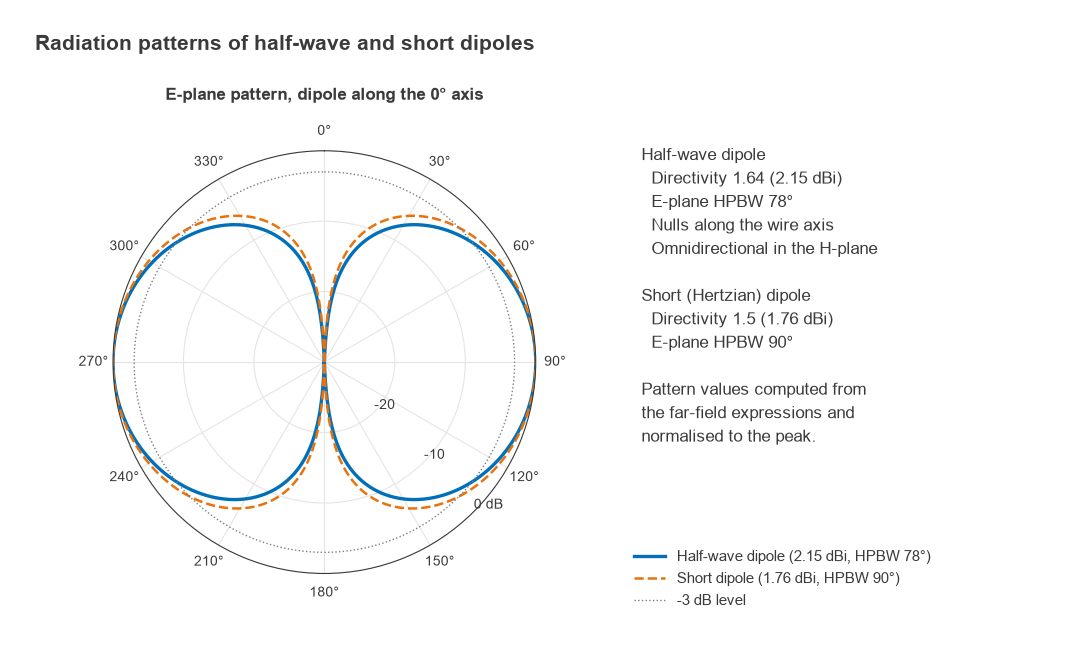
When a single number is quoted it is the maximum value, D₀. Directivity is a property of the pattern shape only. It says nothing about losses, because P_rad is the power that actually leaves the antenna as radiation. Integrating the far-field patterns of the two simplest wire antennas gives the classic values: a short (Hertzian) dipole has D₀ = 1.5, or 1.76 dBi, and a half-wave dipole has D₀ = 1.64, or 2.15 dBi.

Polar E-plane patterns of a half-wave dipole and a short dipole, normalised to the peak — Figure 1: E-plane radiation patterns computed from the far-field expressions. The half-wave dipole has 2.15 dBi directivity and a 78° half-power beamwidth; the short dipole has 1.76 dBi and 90°.

For a pencil-beam antenna with half-power beamwidths θ_E and θ_H in degrees, two approximations are common. Kraus gives D₀ ≈ 41253 / (θ_Eθ_H), and the Tai and Pereira form gives D₀ ≈ 32400 / (θ_Eθ_H). For a beam of 65° by 65° they return 9.9 dBi and 8.9 dBi respectively. The spread shows that these are estimates for comparison, not substitutes for a measured or simulated pattern. Both assume a single main lobe with little energy in sidelobes.

Antenna gain and the role of efficiency

Gain uses the power accepted at the antenna terminals, P_in, instead of the radiated power. Part of P_in is lost as heat in the conductors, the dielectric substrate and any nearby lossy material. The radiation efficiency e_r = P_rad/P_in links the two definitions:

G = e_r × D, or in decibels G(dBi) = D(dBi) + 10log₁₀(e_r)

A lossless antenna has G = D. A small antenna squeezed into a handset, or one sitting close to a battery and a metal chassis, can have efficiency well below 50%, which costs 3 dB or more of gain even when the pattern looks unchanged. Gain is still a passive quantity. An antenna with 6 dBi of gain does not amplify anything; it takes power from some directions and puts it into others.

Realized gain and mismatch

Gain in its formal definition assumes the antenna is matched. In a product, the feed line sees some reflection coefficient Γ, and only a fraction 1 − |Γ|² of the available power enters the antenna. Realized gain includes that loss:

G_realized = (1 − |Γ|²) × e_r × D

The product (1 − |Γ|²) × e_r is the total efficiency, the figure most over-the-air test reports quote. The relationship between Γ, VSWR and mismatch loss is covered on the VSWR and return loss page, and the practical work of bringing Γ down inside an enclosure is covered in antenna matching and tuning.

Worked example: a 2.45 GHz patch

Take a microstrip patch with a simulated directivity of 7.0 dBi, a radiation efficiency of 80%, and a measured VSWR of 2:1 at 2.45 GHz.

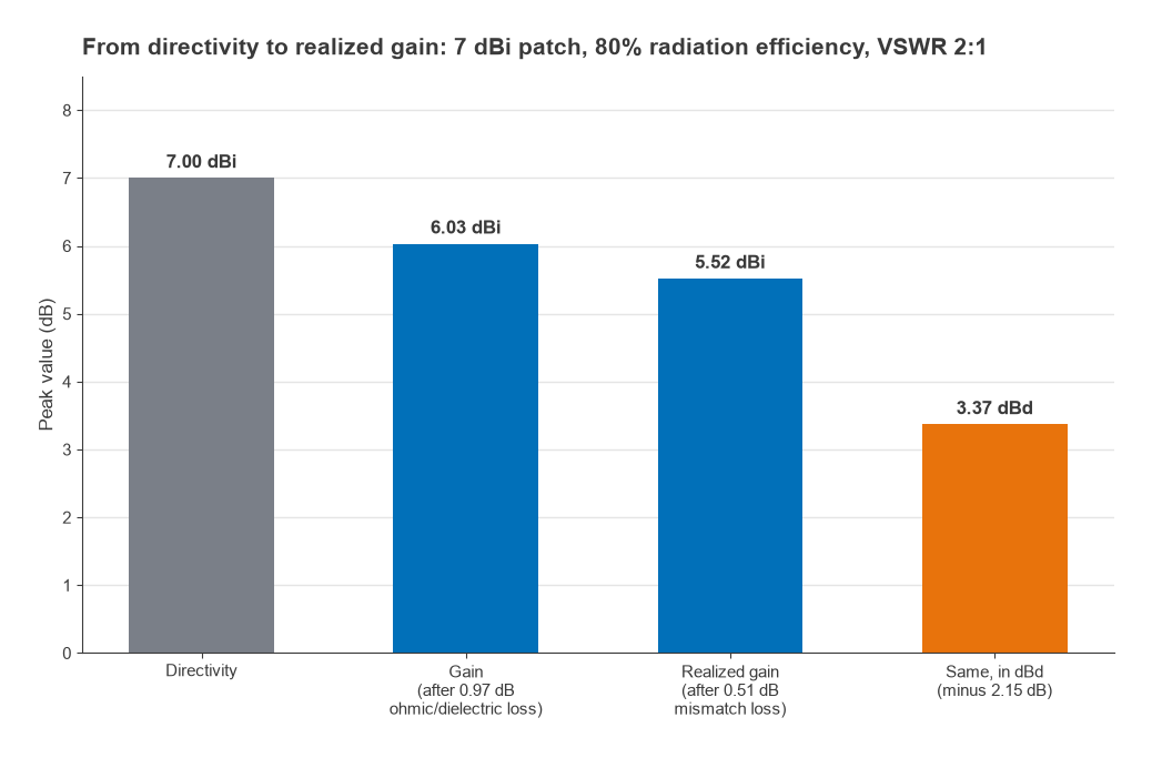
Bar chart of 7.00 dBi directivity, 6.03 dBi gain, 5.52 dBi realized gain and 3.37 dBd for the example patch — Figure 2: From directivity to realized gain for the worked example: 0.97 dB lost to 80% radiation efficiency and 0.51 dB to a 2:1 VSWR mismatch.

Efficiency loss: 10log(0.80) = −0.97 dB, so G = 7.00 − 0.97 = 6.03 dBi.
Reflection: |Γ| = (2 − 1)/(2 + 1) = 0.333, so 1 − |Γ|² = 0.889 and the mismatch loss is 0.51 dB.
Realized gain: 6.03 − 0.51 = 5.52 dBi. Total efficiency is 0.80 × 0.889 = 0.711, or 71%.
Against a half-wave dipole: 5.52 − 2.15 = 3.37 dBd.
With 20 dBm delivered to the feed line, EIRP = 20 + 5.52 = 25.52 dBm in the direction of the peak.

The same realized gain sets the effective aperture, the area over which the antenna collects incoming power when receiving: A_e = Gλ²/4π. At 2.45 GHz, λ = 0.1224 m, and a linear gain of 10^0.552 = 3.56 gives A_e ≈ 42.5 cm². This is the quantity that appears, in another form, in the free-space path loss and Friis equations.

dBi versus dBd

Gain needs a reference antenna. dBi uses the isotropic radiator, which cannot be built but makes the arithmetic of link budgets simple. dBd uses a lossless half-wave dipole, which can be built and was the traditional reference for broadcast and land-mobile antennas. Since the dipole has 2.15 dBi of gain:

G(dBi) = G(dBd) + 2.15

A specification that says only “dB” is ambiguous, and the 2.15 dB difference is large enough to matter in a regulatory EIRP calculation. When comparing datasheets, convert everything to dBi first. ERP, used in some broadcast rules, is referenced to a dipole, so EIRP = ERP + 2.15 dB.

Radiation pattern and beamwidth

The radiation pattern is a plot of relative field strength or power against direction in the far field. Because a full three-dimensional pattern is hard to read, two principal cuts are normally shown: the E-plane, containing the electric field vector and the direction of maximum radiation, and the H-plane, perpendicular to it. Patterns are normalised to the peak and plotted in dB, either on a polar grid or on a rectangular grid of level versus angle.

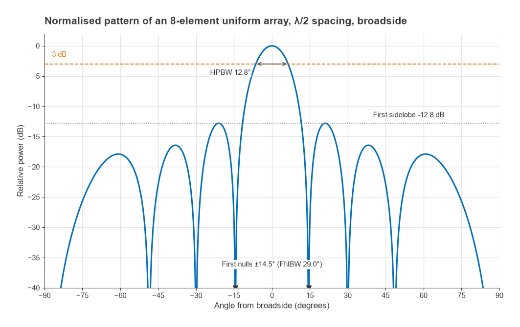
Pattern of an 8-element half-wave spaced array: 12.8 degree beamwidth, nulls at 14.5 degrees, -12.8 dB sidelobes — Figure 3: Normalised array factor of an 8-element uniform broadside array with λ/2 spacing: HPBW 12.8°, first nulls at ±14.5° and first sidelobes at −12.8 dB.

Several numbers are read from a pattern:

Half-power beamwidth (HPBW): the angle between the two points on the main lobe where power is 3 dB below the peak. The half-wave dipole has an E-plane HPBW of 78°; the short dipole has 90°.
First-null beamwidth (FNBW): the angle between the first nulls either side of the main lobe.
Sidelobe level (SLL): the level of the highest sidelobe relative to the main lobe, in dB.
Front-to-back ratio: the ratio of peak gain to gain in the opposite direction, important for sector antennas and for rejecting interference from behind.

An array of N identical elements with uniform excitation and spacing d shows how these quantities trade against each other. For broadside radiation the array factor is |sin(Nψ/2) / (N sin(ψ/2))| with ψ = kd sinθ. For N = 8 and d = λ/2 the exact HPBW is 12.8°, close to the approximation 0.886λ/(Nd) radians, which gives 12.7°. The first nulls fall at sin⁻¹(2/N) = ±14.5°, and the first sidelobe sits 12.8 dB below the peak, approaching the familiar 13.3 dB limit as N grows. Tapering the excitation lowers the sidelobes at the cost of a wider main beam. The phased array design and beamforming pages take this further.

Polarization

Polarization describes the path traced by the tip of the electric field vector in the direction of maximum radiation. A dipole or monopole is linearly polarized. Two orthogonal linear components fed 90° apart produce circular polarization, right-hand or left-hand depending on the sense of rotation. In practice most antennas are elliptically polarized to some degree, and the axial ratio, the ratio of major to minor axis of the polarization ellipse, measures how close a nominally circular antenna comes to the ideal of 0 dB.

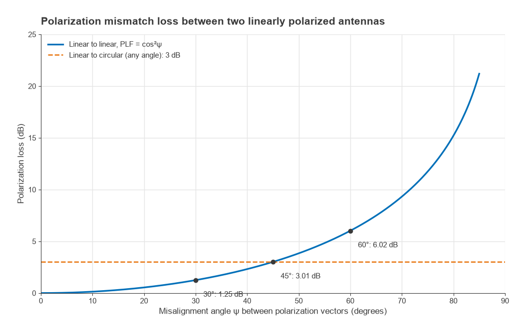
When transmit and receive polarizations differ, only part of the incident power couples into the receiving antenna. For two linear antennas misaligned by angle ψ the polarization loss factor is PLF = cos²ψ. A 30° twist costs 1.25 dB, 45° costs 3.01 dB and 60° costs 6.02 dB. A linear antenna receiving a circular wave loses 3 dB regardless of orientation, which is one reason satellite and GNSS links use circular polarization: the receive antenna does not need to know which way is up. Cross-polar discrimination, the ratio of co-polar to cross-polar gain, is the matching specification on a dual-polarized antenna.

Impedance bandwidth and other specifications

An antenna is also a circuit element. Its input impedance varies with frequency, and the impedance bandwidth is the range over which the match meets a stated limit, commonly a return loss of 10 dB (VSWR about 1.9:1) for compact antennas or 14 to 20 dB for infrastructure antennas. Pattern bandwidth, the range over which gain and beamwidth stay within limits, can be narrower or wider than the impedance bandwidth. Other datasheet entries include maximum input power, which depends on heating and on voltage breakdown at sharp edges, and passive intermodulation for antennas shared between transmit and receive.

For printed antennas, all of these parameters change once the antenna is mounted on a real board with a ground plane of finite size and nearby components. The PCB antenna design and patch antenna design pages show how geometry sets resonance, bandwidth and directivity in practice.

Frequently asked questions

What is antenna gain in dBi?

It is the gain of the antenna relative to an ideal isotropic radiator, expressed in decibels. An antenna with 6 dBi produces, in its best direction, four times the power density an isotropic source would produce from the same input power. The figure includes radiation efficiency but, unless stated as realized gain, not mismatch loss.

What is the difference between gain and directivity?

Directivity describes only the shape of the radiation pattern and is referenced to radiated power. Gain is referenced to the power accepted at the antenna input, so it includes conductor and dielectric losses. The two are linked by G = e_r × D, and they are equal only for a lossless antenna.

How do I convert dBd to dBi?

Add 2.15 dB. A half-wave dipole has a gain of 2.15 dBi, so an antenna quoted at 3 dBd has 5.15 dBi. Going the other way, subtract 2.15 dB.

Does a higher-gain antenna always perform better?

No. Higher gain comes from a narrower beam, so it helps only when the antenna is pointed at the other end of the link. A mobile device that can be held in any orientation usually benefits more from a broad pattern and high efficiency than from peak gain.