Pi and T Matching Networks

Pi and T matching networks are three-element lumped matching circuits that let the designer choose the network Q, and therefore the bandwidth, instead of accepting the fixed Q of a two-element L-network. Use a pi or T instead of an L when you need a narrower bandwidth, more harmonic suppression, or component values that are easier to build. The usual design method splits the network into two L-sections that meet at an imaginary “virtual resistance”.

Pi and T networks build directly on the L-network, and both belong to the broader topic of impedance matching. This page shows how to design them step by step, how to pick Q, and why a low-pass pi is the classic output network for power amplifiers.

Why add a third element

An L-network matching R_low to R_high has exactly one Q for each topology:

Q_L = √(R_high/R_low − 1)

That Q sets the bandwidth, the harmonic attenuation and the component values together. A 4:1 ratio gives Q = 1.73, which is broadband but provides little filtering. A third element adds one degree of freedom, so Q can be set anywhere above the L-network minimum. The pi network has a shunt element at each port and one series element in the middle; the T network is the dual, with a series element at each port and one shunt element in the middle.

The virtual resistance method

A pi or T network can be viewed as two L-networks connected back to back. The first L transforms one port to an intermediate resistance R_v, and the second transforms R_v to the other port. R_v never appears as a physical resistor; it is the resistance seen at the junction between the two halves.

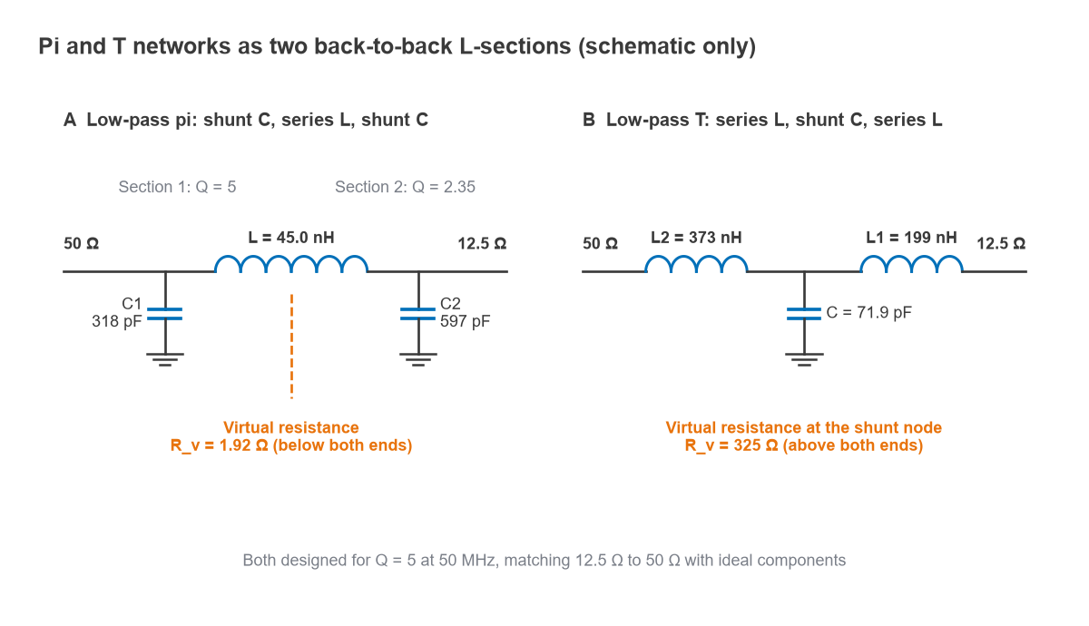
Low-pass pi and T matching networks with component values and the virtual resistance marked — Figure 1: Low-pass pi and T networks for 12.5 Ω to 50 Ω at 50 MHz with Q = 5 (schematic only).

Pi network: each L has its shunt element at the outer port and its series element facing the middle, so R_v must be lower than both terminating resistances. For a chosen Q on the higher-resistance side, R_v = R_high/(Q² + 1).
T network: each L has its series element at the outer port and its shunt element in the middle, so R_v must be higher than both. For a chosen Q on the lower-resistance side, R_v = R_low(Q² + 1).

The network Q is normally taken as the higher of the two section Qs. That is the section that dominates the bandwidth, and it is the one the designer specifies.

Design steps for a pi network

Choose the loaded Q. It must exceed the L-network value √(R_high/R_low − 1).
Compute R_v = R_high/(Q² + 1).
High side: shunt reactance X_p1 = R_high/Q and series reactance X_s1 = Q × R_v.
Low side: Q₂ = √(R_low/R_v − 1), shunt reactance X_p2 = R_low/Q₂ and series reactance X_s2 = Q₂ × R_v.
Combine the two series reactances into one element: X_s = X_s1 + X_s2 if they are the same type.
Convert to component values with L = X/(2πf) and C = 1/(2πfX), then simulate with real parts.

The T network follows the same steps with the roles reversed: series reactances X_s = Q × R at each outer port, shunt reactances R_v/Q in the middle, and the two shunt elements combined in parallel.

Worked example: 12.5 Ω to 50 Ω at 50 MHz

Suppose a transistor stage needs a 12.5 Ω load at 50 MHz and the output must drive a 50 Ω system. The L-network Q would be √(50/12.5 − 1) = 1.73. Choose a low-pass pi with Q = 5 for more selectivity.

R_v = 50/(5² + 1) = 50/26 = 1.923 Ω.
50 Ω side: X_p1 = 50/5 = 10.0 Ω, so C1 = 1/(2π × 50 MHz × 10.0) = 318 pF. X_s1 = 5 × 1.923 = 9.62 Ω.
12.5 Ω side: Q₂ = √(12.5/1.923 − 1) = √5.5 = 2.345. X_p2 = 12.5/2.345 = 5.33 Ω, so C2 = 597 pF. X_s2 = 2.345 × 1.923 = 4.51 Ω.
Series inductor: X_s = 9.62 + 4.51 = 14.13 Ω, so L = 14.13/(2π × 50 MHz) = 45.0 nH.

For the T version at the same Q, R_v = 12.5 × 26 = 325 Ω. The 12.5 Ω side needs a series reactance of 5 × 12.5 = 62.5 Ω (199 nH) and a shunt reactance of 325/5 = 65.0 Ω. The 50 Ω side has Q₂ = √(325/50 − 1) = 2.345, a series reactance of 117.3 Ω (373 nH) and a shunt reactance of 138.6 Ω. The two shunt reactances in parallel give 44.2 Ω, a single 71.9 pF capacitor.

Network (12.5 Ω to 50 Ω, 50 MHz)	Components	−20 dB return-loss band	\|S₂₁\| at 100 MHz	\|S₂₁\| at 150 MHz
Low-pass L, Q = 1.73	Shunt 110 pF, series 68.9 nH	46.53 to 53.24 MHz (13.4%)	−7.8 dB	−15.7 dB
Low-pass pi, Q = 3	191 pF, 67.2 nH, 312 pF	48.48 to 51.40 MHz (5.8%)	−19.7 dB	−31.5 dB
Low-pass pi, Q = 5	318 pF, 45.0 nH, 597 pF	49.24 to 50.72 MHz (3.0%)	−26.0 dB	−38.0 dB
Low-pass pi, Q = 10	637 pF, 23.5 nH, 1254 pF	49.65 to 50.34 MHz (1.4%)	−32.8 dB	−44.8 dB
Low-pass T, Q = 5	373 nH, 71.9 pF, 199 nH	49.24 to 50.72 MHz (3.0%)	−26.0 dB	−38.0 dB

All figures in the table come from a circuit simulation of ideal components, with the input referenced to 50 Ω and the output terminated in 12.5 Ω. The low-pass pi and low-pass T at the same Q are duals and give identical responses here; the choice between them is about practical component values and DC paths.

Choosing Q: bandwidth and loss

Bandwidth falls roughly in proportion to 1/Q. In the example, raising Q from the L-network minimum of 1.73 to 3, 5 and 10 shrinks the 20 dB return-loss bandwidth from 13.4% to 5.8%, 3.0% and 1.4%. A narrow match is useful when the network must also filter, and harmful when the system has to tolerate component tolerances or cover a band.

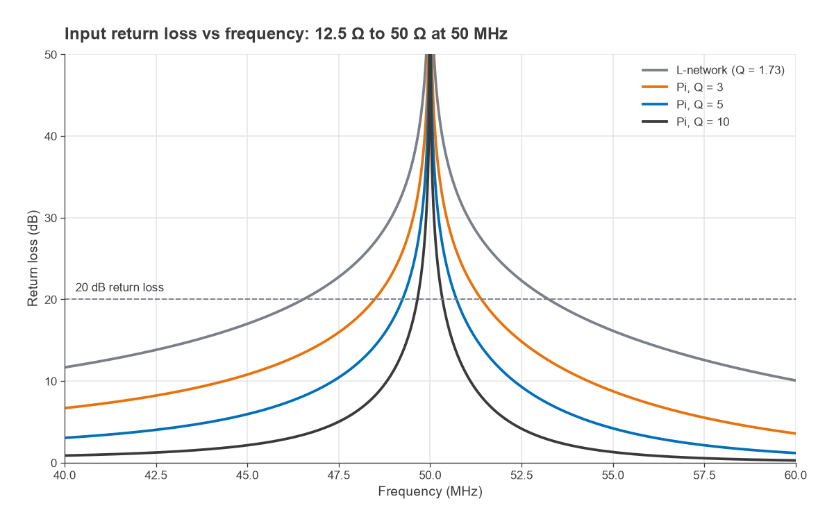
Return loss versus frequency for an L-network and pi networks with Q of 3, 5 and 10 — Figure 2: Return loss of the 50 MHz match. The 20 dB bandwidth falls from 13.4% (L) to 5.8%, 3.0% and 1.4% for Q = 3, 5 and 10.

Loss grows with Q because circulating currents grow with Q. For small losses the insertion loss of a pi network is approximately

IL ≈ 4.34 (Q₁ + Q₂)(1/Q_u,L + 1/Q_u,C) dB

where Q_u is the unloaded Q of the inductors and capacitors. With an inductor Q_u of 100 and capacitor Q_u of 500, the estimate gives 0.22 dB at Q = 3, 0.38 dB at Q = 5 and 0.78 dB at Q = 10, against 0.09 dB for the L-network. A simulation with the same lossy parts gives 0.22, 0.38 and 0.75 dB. At a power amplifier output, 0.38 dB is about 8% of the output power turned into heat in the matching network, which is why designers rarely push Q higher than the harmonic or bandwidth requirement demands. The Q-factor page covers unloaded and loaded Q in more depth.

Practical guidance for a first design: start with Q between about 1.5 and 3 times the L-network minimum, then adjust to meet the harmonic and bandwidth requirements. Very high Q also makes the match sensitive to component tolerance, because a few percent change in a reactance moves the resonance by a significant fraction of the bandwidth.

Harmonic suppression of pi networks

A low-pass pi is a third-order low-pass filter. Above the design frequency, the series inductor’s reactance rises while both shunt capacitors’ reactances fall, so attenuation rises at about 18 dB per octave well above resonance. An L-network is only second order, with about 12 dB per octave. Figure 3 shows the effect for the 50 MHz example: at the second harmonic the Q = 5 pi attenuates by 26.0 dB against 7.8 dB for the L-network, and at the third harmonic by 38.0 dB against 15.7 dB.

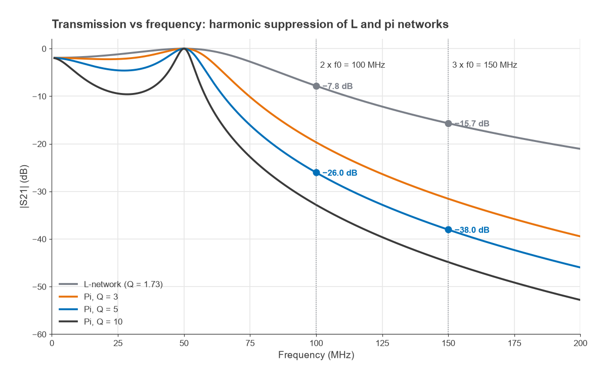
Transmission versus frequency showing harmonic attenuation of L and pi matching networks — Figure 3: The Q = 5 pi attenuates 26.0 dB at 100 MHz and 38.0 dB at 150 MHz, against 7.8 dB and 15.7 dB for the L-network.

That is why the pi network has been the standard tank and output network for transmitters for most of radio history. It matches the device, filters its harmonics, and puts a capacitor across each port, which conveniently absorbs the output capacitance of the transistor or tube on one side and gives a low-impedance shunt path for harmonics on the other. A high-pass pi or T (series capacitors, shunt inductors) attenuates below the design frequency instead, which suits interstage matching where low-frequency gain must be suppressed or where the shunt inductors double as bias feeds.

Harmonic attenuation from a single matching network is rarely enough to meet a spurious-emission limit on its own, which is typically tens of decibels below the carrier. A separate low-pass filter usually follows; see LC filter design for the method.

Pi or T: practical selection

Absorbing device capacitance: a pi with shunt capacitors at the ports absorbs the output capacitance of a transistor or the input capacitance of the next stage. A T with series inductors absorbs series lead and package inductance.
Component values: a pi between low resistances tends to need large capacitors and a small inductor, as the 597 pF and 45 nH in the example show. A T between the same resistances needs larger inductors and a small capacitor. Pick the version whose values are realizable with good Q at the frequency.
DC paths: low-pass forms pass DC through the series element; high-pass forms block it. Choose according to how bias is fed.
Parasitics: at high frequencies, pad capacitance favours shunt capacitors at the ports, and the pi often maps more naturally onto a printed layout.

At microwave frequencies the same ideas carry over to distributed circuits: the quarter-wave transformer and stub matching replace lumped parts with line sections, and the Smith chart shows a pi network as two L-network paths meeting at the constant-Q contour chosen by the designer.

Frequently asked questions

When use a pi network instead of an L?

Use a pi when the L-network’s fixed Q gives too much bandwidth or too little harmonic suppression, or when its component values are impractical. A pi lets you set Q above the L-network minimum and adds a third pole of low-pass filtering.

What is the virtual resistance in a pi network?

It is the intermediate resistance where the two back-to-back L-sections meet. For a pi it is lower than both port resistances and equals R_high/(Q² + 1); for a T it is higher than both and equals R_low(Q² + 1).

What Q should I choose for a pi matching network?

Choose the lowest Q that meets the harmonic and selectivity requirements. Higher Q narrows bandwidth, raises loss and increases sensitivity to component tolerances. A starting point of 1.5 to 3 times the L-network Q is common.