

A patch antenna is a resonant printed antenna: a flat metal rectangle on a grounded dielectric substrate that radiates from the fringing fields at its two open edges. Its dimensions follow from three inputs, the frequency, the substrate permittivity and the thickness. The width W is chosen for efficient radiation, and the length L is set slightly shorter than half a wavelength in the substrate to allow for fringing. The feed position then sets the input impedance.
This page gives the standard transmission-line-model equations, works a 2.45 GHz FR-4 example by hand, explains the inset feed used to reach 50 Ω, and ends with a calculator. It belongs to the antennas section of the RF design guide; the general terms used here, such as gain, directivity and bandwidth, are defined in antenna parameters.
How a Patch Antenna Works
The patch and ground plane form a short section of wide microstrip line, open at both ends. At resonance the line is about half a guided wavelength long, so the voltage is maximum and of opposite sign at the two ends, and zero in the middle. The electric field that fringes out beyond each end points the same way in the plane of the substrate, and the two fringing regions act as a pair of radiating slots of width W separated by L. Their fields add broadside to the board, which is why a patch radiates mainly away from the ground plane with a gain typically around 6 to 8 dBi on low-loss material.
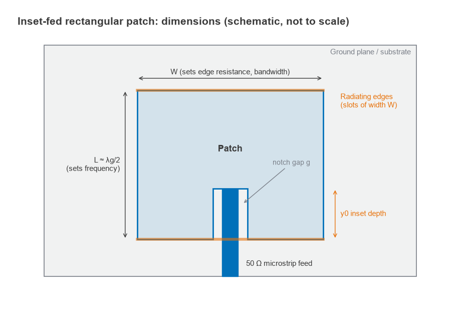
The transmission line model treats each radiating edge as a slot with a conductance G1 and a small susceptance, connected by a length L of line. It is less exact than a cavity model or a full-wave simulation, but it predicts the resonant length to within a few percent on thin substrates and gives the designer the right starting dimensions.
Patch Width and Length Equations
Step 1: width
A practical width that gives good radiation efficiency without exciting higher-order modes is
W = (c / 2fr) · √[2 / (εr + 1)]
The width is not critical for resonance. A wider patch has higher radiation conductance, so a lower edge resistance, and slightly more bandwidth and gain. A much wider patch can support a transverse mode near the operating frequency.
Step 2: effective permittivity
Part of the field under the patch is in air, so the wave sees an effective permittivity between 1 and εr. For W/h > 1:
εeff = (εr + 1)/2 + (εr − 1)/2 · (1 + 12h/W)−1/2
This is the same expression used for wide microstrip lines in the microstrip calculator.
Step 3: fringing length extension
The fringing field makes each open end look electrically longer by ΔL, given by the Hammerstad expression:
ΔL = 0.412h · [(εeff + 0.3)(W/h + 0.264)] / [(εeff − 0.258)(W/h + 0.8)]
Step 4: physical length
The physical length is half the guided wavelength minus the two extensions:
L = c / (2fr√εeff) − 2ΔL
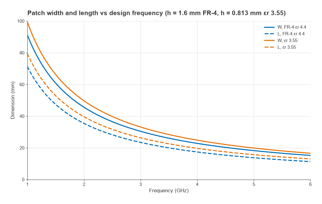
Figure 3 shows how both dimensions scale roughly as 1/f across 1 to 6 GHz on two common substrates.
Worked Example: 2.45 GHz Patch on FR-4
Design for fr = 2.45 GHz on FR-4 with εr = 4.4 and h = 1.6 mm.
- Free-space wavelength: λ0 = c/f = 122.4 mm.
- Width: W = (122.4/2) · √(2/5.4) = 37.2 mm.
- Effective permittivity: W/h = 23.3, so εeff = 2.7 + 1.7 · (1 + 12/23.3)−1/2 = 4.08.
- Length extension: ΔL = 0.74 mm.
- Length: L = 122.4 / (2 · √4.08) − 2 · 0.74 = 30.29 − 1.48 = 28.8 mm.
The patch is therefore 37.2 mm wide and 28.8 mm long. Ignoring fringing and using εr directly would give 29.2 mm and tune the antenna about 1.4 % low. The more serious uncertainty on FR-4 is the permittivity itself, which varies between laminates and with frequency. Keeping the same 37.2 × 28.8 mm patch, εr = 4.2 moves the resonance up to 2.51 GHz and εr = 4.6 moves it down to 2.40 GHz, a shift of about ±2.2 %. That is larger than the bandwidth calculated below, so the first prototype is normally trimmed after measurement, and production designs often move to a laminate with a controlled permittivity, as discussed in FR-4 vs Rogers.
Inset Feed for a 50 Ω Match
Fed at the centre of a radiating edge, a patch presents a high resistance, typically 200 to 300 Ω or more. In the transmission line model the edge resistance is
Rin(0) = 1 / [2(G1 + G12)]
where G1 is the radiation conductance of one slot and G12 the mutual conductance between the two slots, both found by numerical integration of the slot radiation patterns. For the FR-4 example, G1 = 0.97 mS and G12 = 0.59 mS, so Rin(0) = 321 Ω.
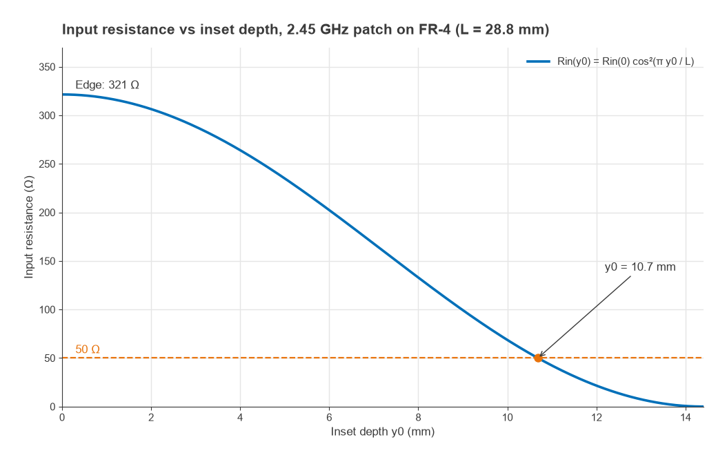
The voltage along the resonant patch varies as cos(πy/L) and the current as sin(πy/L), so the resistance seen by a feed moved a distance y0 in from the edge falls as
Rin(y0) = Rin(0) · cos2(πy0/L), so y0 = (L/π) · arccos√(Z0/Rin(0))
For Z0 = 50 Ω: y0 = (28.8/π) · arccos√(50/321) = 10.7 mm. The 50 Ω microstrip on 1.6 mm FR-4 is about 3.1 mm wide. It runs into a notch cut into the patch, with a small gap on each side, typically around 0.5 to 1 mm, so that it does not touch the patch until it reaches the feed point. The notch disturbs the current slightly and the cos2 law is an approximation, so the optimum inset found in an EM simulation or on the bench is usually somewhat different from the hand value. Figure 2 shows the curve; near 50 Ω it is steep, about 25 Ω per millimetre, which is why the inset is tuned in fine steps.
Other feeds avoid the notch. A coaxial probe from below is placed at the same y0 and leaves the top layer clean, at the cost of probe inductance on thick substrates. A quarter-wave transformer from the edge, described in quarter-wave transformer, needs a line of √(50 × 321) = 127 Ω, which is narrow on FR-4 but realisable. Aperture and proximity coupling use a second layer and give more bandwidth. Any residual mismatch can be trimmed with the techniques in antenna matching.
Bandwidth and Substrate Choice
A patch is a high-Q resonator, and its bandwidth is narrow. A widely used approximation for the VSWR < 2 bandwidth of a thin rectangular patch is
BW ≈ 3.77 · [(εr − 1)/εr2] · (W/L) · (h/λ0)
For the FR-4 example this gives 1.12 %, or about 27 MHz, enough for the 2.400 to 2.4835 GHz band only if the patch is centred within a few megahertz and the reflection target is relaxed. The formula covers radiation only. FR-4’s dielectric loss lowers the Q, so a measured FR-4 patch is usually somewhat wider in bandwidth than predicted, but the extra bandwidth comes from heat, not radiation, and gain falls accordingly.
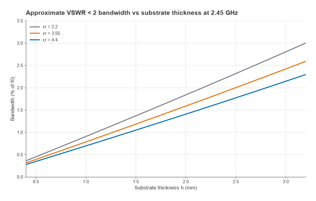
Bandwidth grows almost linearly with h/λ0 and is larger for lower permittivity, as Figure 4 shows. Doubling FR-4 thickness to 3.2 mm raises it to 2.3 %; a 1.575 mm PTFE substrate with εr = 2.2 gives 1.44 % from a larger 48.4 × 40.5 mm patch. Thick substrates also launch more surface waves and make the probe or inset feed more inductive, which limits how far the thickness can be pushed.
| Substrate | εr | h (mm) | fr (GHz) | W (mm) | L (mm) | Rin(0) (Ω) | 50 Ω inset y0 (mm) | BW (%) |
|---|---|---|---|---|---|---|---|---|
| FR-4 | 4.4 | 1.6 | 2.45 | 37.2 | 28.8 | 321 | 10.7 | 1.12 |
| Hydrocarbon ceramic laminate | 3.55 | 0.813 | 2.45 | 40.6 | 32.3 | 290 | 11.8 | 0.64 |
| PTFE | 2.2 | 1.575 | 2.45 | 48.4 | 40.5 | 245 | 14.2 | 1.44 |
| FR-4 | 4.4 | 1.6 | 5.8 | 15.7 | 11.7 | 317 | 4.3 | 2.75 |
| Hydrocarbon ceramic laminate | 3.55 | 0.813 | 5.8 | 17.1 | 13.5 | 288 | 4.9 | 1.53 |
The ground plane should extend beyond the patch by a few substrate thicknesses on every side; a common rule of thumb is about 6h plus the patch dimension. A smaller ground plane raises back radiation and shifts the resonance, which matters when the patch is integrated on a product board as described in PCB antenna design.
Patch Antenna Calculator
The calculator applies the equations above, including the numerical integration for the edge resistance. Results are starting dimensions for simulation and prototyping, not final values.
Frequently Asked Questions
How do you calculate patch antenna dimensions?
Compute the width from W = (c/2f)√[2/(εr+1)], then the effective permittivity and the fringing extension ΔL, and finally L = c/(2f√εeff) − 2ΔL. On 1.6 mm FR-4 at 2.45 GHz this gives 37.2 × 28.8 mm.
Where should a patch antenna be fed?
At the point along the length where the resistance equals the feed impedance. Using Rin(y0) = Rin(0)cos2(πy0/L), a 50 Ω feed on the FR-4 example sits about 10.7 mm in from the radiating edge, before tuning.
Why is my patch antenna off frequency?
The usual causes are an inaccurate substrate permittivity, a small ground plane, nearby enclosure parts and etching tolerance on L. On FR-4 a ±0.2 change in εr shifts a 2.45 GHz patch by about ±2 %, more than its bandwidth.
How can I increase patch antenna bandwidth?
Use a thicker or lower-permittivity substrate, or a foam or air dielectric. Stacked patches and aperture-coupled feeds widen it further at the cost of an extra layer.
Related Topics
The antennas hub links every antenna topic. Patches are the building block of the arrays covered in phased array design and in antennas and propagation in radio design, Part 17 of Radio Architectures. The feed and transformer calculations connect to impedance matching and the Smith chart, and the received power of a finished antenna follows from free-space path loss.