

Grounded coplanar waveguide (GCPW) is a planar transmission line in which a signal strip runs between two ground planes on the same layer, separated by gaps, with a further ground plane underneath the substrate and rows of vias tying all the grounds together. Its impedance is set mainly by the strip width and the gap, which makes it easier than microstrip to hold 50 Ω with narrow traces and to isolate neighbouring lines at high frequencies.
Coplanar lines are the usual choice for millimetre-wave boards, connector launches, probe pads and densely packed RF layouts. This page gives the conformal-mapping equations for CPW and GCPW, shows how the impedance depends on the gap, provides a calculator, and works through a 50 Ω design on a common low-loss laminate including the via fence. It belongs to the transmission lines section of the RF design guide, alongside microstrip and stripline.
CPW and GCPW Geometry
Conventional coplanar waveguide (CPW) has a centre strip of width S and two coplanar grounds separated from it by gaps W, all on the top of a substrate of height h and relative permittivity εr. There is no metal underneath. The field runs mainly across the two gaps, half in the substrate and half in the air above, so the effective permittivity is close to (εr + 1)/2 for a thick substrate.
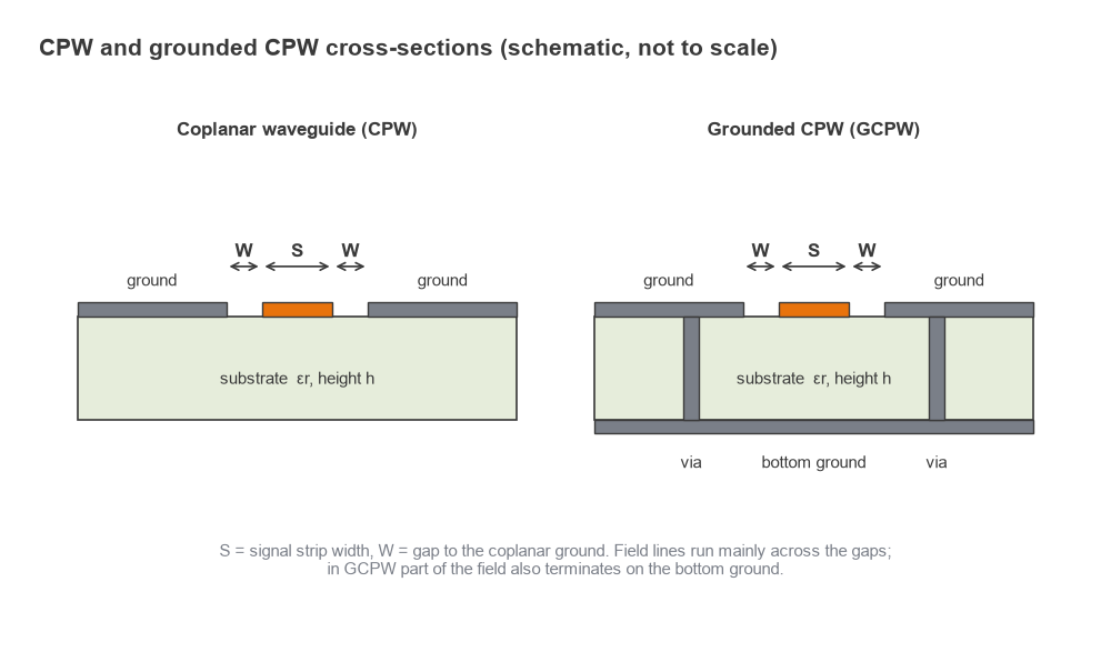
On a printed circuit board there is almost always a ground plane on the next layer, so the practical structure is grounded or conductor-backed CPW. Part of the field now terminates on the bottom ground, which lowers the impedance and raises the effective permittivity compared with plain CPW. The top grounds must be tied to the bottom ground with vias along both sides of the line; without them the top grounds can float at different potentials and support unwanted modes. Comparisons with other line types are in types of transmission lines.
Characteristic Impedance Equations
Closed-form CPW and GCPW equations come from conformal mapping and are expressed with the complete elliptic integral of the first kind, K(k). Define the modulus k0 = S/(S + 2W) and the complementary modulus k′ = √(1 − k2). For the quasi-TEM mode with zero-thickness conductors and infinitely wide coplanar grounds:
CPW on a finite substrate
k1 = sinh(πS/4h) / sinh(π(S + 2W)/4h)
εeff = 1 + [(εr − 1)/2] × [K(k1)/K(k1′)] × [K(k0′)/K(k0)]
Z0 = (30π/√εeff) × K(k0′)/K(k0)
Grounded CPW
k3 = tanh(πS/4h) / tanh(π(S + 2W)/4h)
q = [K(k3)/K(k3′)] / [K(k0)/K(k0′)]
εeff = (1 + εrq)/(1 + q)
Z0 = (60π/√εeff) × 1 / [K(k0)/K(k0′) + K(k3)/K(k3′)]
The GCPW expression treats the line as two capacitances in parallel: one to the coplanar grounds through air and substrate, and one to the bottom ground through the substrate. These forms appear in standard references on coplanar lines and are usually quoted as good to a few percent when the gap is not much larger than the substrate height and the grounds are at least several times the gap in width. Conductor thickness lowers Z0 by adding sidewall capacitance in the gaps, which matters more for CPW than for microstrip because the gaps are narrow. Solder mask over the gaps also lowers Z0 by a few ohms. For final dimensions, confirm with a 2D field solver or an EM simulation.
How Z0 Depends on the Gap
Narrowing the gap increases the capacitance to the coplanar grounds and lowers Z0; widening it raises Z0 until the coplanar grounds stop mattering and the line behaves like a microstrip over the bottom ground. In GCPW the impedance therefore saturates at large gaps, while in CPW without a bottom ground it keeps rising. The useful design range is where the gap is smaller than about the substrate height, because that is where the gap actually controls the impedance.
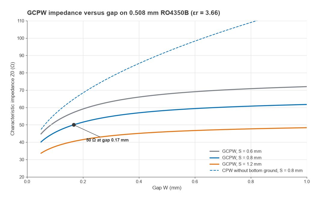
The table gives the gap for 50 Ω for several strip widths, from the GCPW equations above with zero-thickness copper. Treat the permittivities as typical design values and confirm them with your fabricator.
| Substrate | εr | h (mm) | Strip S (mm) | Gap W for 50 Ω (mm) | εeff |
|---|---|---|---|---|---|
| RO4350B | 3.66 | 0.508 | 0.6 | 0.086 | 2.45 |
| RO4350B | 3.66 | 0.508 | 0.8 | 0.167 | 2.54 |
| RO4350B | 3.66 | 0.508 | 1.0 | 0.382 | 2.68 |
| FR-4, 2-layer | 4.3 | 1.6 | 1.0 | 0.136 | 2.70 |
| FR-4, 2-layer | 4.3 | 1.6 | 1.5 | 0.244 | 2.75 |
| FR-4, 2-layer | 4.3 | 1.6 | 2.0 | 0.423 | 2.84 |
Note how sensitive the gap becomes as the strip approaches the microstrip 50 Ω width (1.12 mm on 0.508 mm RO4350B): going from S = 0.8 mm to 1.0 mm more than doubles the required gap. Designs tolerate etch variation better when the strip is clearly narrower than the microstrip width, so the gap does real work.
Grounded Coplanar Waveguide Calculator
Enter the strip width, gap, substrate height and permittivity to calculate Z0 and εeff, or enter a target impedance to find the gap. The frequency is used for the guided wavelength and the suggested via pitch.
| Gap W | – |
| Characteristic impedance Z0 | – |
| Effective permittivity εeff | – |
| Guided wavelength λg at f | – |
| Via pitch, λ/20 to λ/10 in the dielectric | – |
Design Procedure and Worked Example
Design a 50 Ω GCPW line for 10 GHz on 0.508 mm RO4350B (εr = 3.66) with a bottom ground on the next layer.
- Choose the strip width. It should be narrower than the 1.12 mm microstrip width so that the gap controls the impedance, and wide enough for low conductor loss and for the component pads it connects to. Take S = 0.8 mm.
- Find the gap. Solving the GCPW equation gives W = 0.167 mm; round to 0.17 mm, which must be within the fabricator's minimum gap. Then εeff = 2.54.
- Check the tolerance. An etch variation of ±0.025 mm in the gap moves Z0 from 48.6 Ω to 51.2 Ω, about ±1.3 Ω. Gaps of 0.15 and 0.20 mm give 49.1 Ω and 51.6 Ω.
- Compute the wavelengths. The guided wavelength is λg = c/(f√εeff) = 299.8/(10 × √2.538) = 18.8 mm, so a quarter-wave section is 4.70 mm. The wavelength in the bulk dielectric is λd = c/(f√εr) = 15.7 mm.
- Size the via fence (next section): pitch between 0.78 and 1.57 mm, rows close to the gap edges.
- Add copper thickness, solder mask and plating to a field-solver model, adjust the gap if needed, and simulate the connector launch.
Via Fence Spacing Rule
The vias along a GCPW line hold the top grounds at the potential of the bottom ground and block parallel-plate and substrate modes from propagating between the two metal layers. A common rule of thumb places the vias no more than λ/10 to λ/20 apart along the line, where λ is the wavelength at the highest frequency of interest. Using the wavelength in the bulk dielectric rather than the guided wavelength is the conservative choice, because it is the shorter of the two.
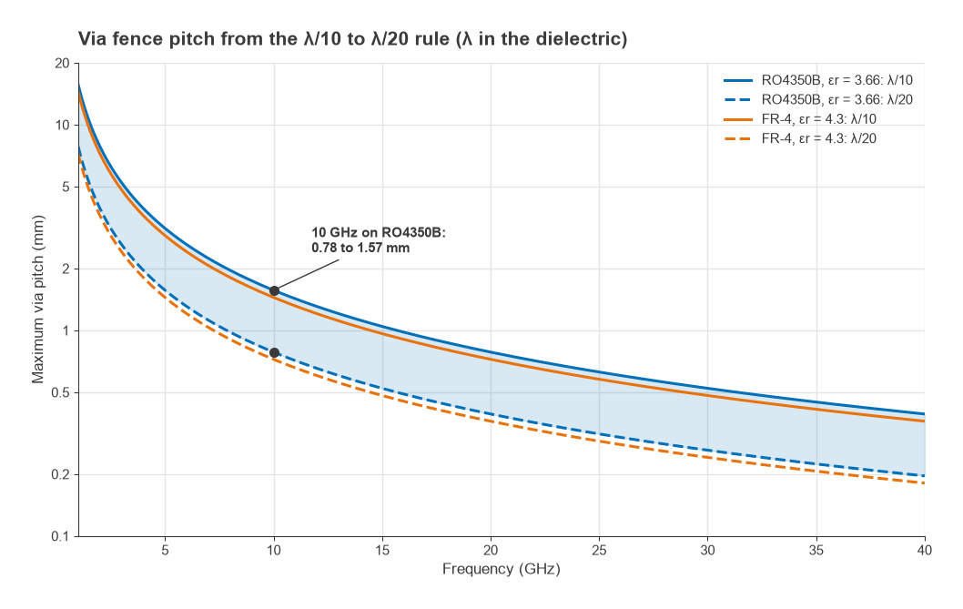
For the worked example at 10 GHz, λd = 15.7 mm gives a pitch of 0.78 to 1.57 mm. At 28 GHz the same rule gives 0.28 to 0.56 mm, and at 40 GHz 0.20 to 0.39 mm, which approaches the minimum drill-to-drill spacing of many processes. On FR-4 (εr ≈ 4.3) the λ/20 limit is slightly tighter: 0.72 mm at 10 GHz.
The distance between the two via rows matters as well. The grounded channel between the rows behaves like a dielectric-filled waveguide whose lowest mode has a cutoff of roughly c/(2a√εr), where a is the row spacing. With via centres 0.4 mm from each gap edge, a = 0.8 + 2 × 0.17 + 2 × 0.4 = 1.94 mm and the cutoff is about 40 GHz, comfortably above a 10 GHz design. Placing vias far from the gap, or leaving wide unstitched ground areas, lowers this cutoff and can create resonances inside the band. The same principles apply to ground stitching elsewhere on the board, covered in grounding and via stitching.
GCPW vs Microstrip
- Isolation: grounded copper and vias on both sides of every line reduce coupling to neighbouring lines and to the cavity of a shield can.
- Impedance freedom: the gap is a second variable, so a thin strip can be 50 Ω on a thick substrate, matching component pads and connector pins more closely.
- Dispersion and radiation: the field is more tightly confined, so GCPW generally shows less dispersion and radiation at millimetre-wave frequencies than an open microstrip.
- Costs: narrow gaps are sensitive to etch tolerance, the via fences take area, and conductor loss can be slightly higher because current crowds at the gap edges.
Below a few gigahertz on cost-sensitive boards, microstrip with good ground stitching is usually adequate. Above roughly 10 GHz, and for any line that has to pass close to other circuitry, GCPW is the common choice. Laminate choice is discussed in FR-4 vs Rogers, and millimetre-wave layout in mmWave radio architectures.
Frequently Asked Questions
What is grounded coplanar waveguide?
It is a coplanar waveguide with an additional ground plane under the substrate, connected to the coplanar grounds by vias. The signal strip is referenced to grounds on both sides and below, and its impedance depends on the strip width, the gap and the substrate.
Why use GCPW over microstrip?
GCPW confines the field more tightly, which improves isolation and reduces radiation and dispersion at high frequencies. It also lets a narrow strip reach 50 Ω, which makes transitions to connectors, probes and small components cleaner.
What gap gives 50 Ω?
It depends on the strip width and stackup. On 0.508 mm RO4350B a 0.8 mm strip needs a gap of about 0.17 mm; on 1.6 mm FR-4 a 1.0 mm strip needs about 0.14 mm. Use the calculator, then confirm with a field solver that includes copper thickness and solder mask.
How far apart should the vias be?
A common rule is λ/10 to λ/20 at the highest frequency of interest, using the wavelength in the dielectric. At 10 GHz on RO4350B that is about 0.8 to 1.6 mm. Keep the rows close to the gap edges as well.
Related Topics
The transmission line theory hub links all the line types. Transmission line parameters and wave propagation cover the underlying theory, the microstrip calculator handles the simpler line, and RF PCB layout puts all of them on a real board. More tools are on the RF calculators page.