

VNA calibration is the procedure that measures a set of known standards at the ends of the test cables so the analyzer can solve for, and then remove, its own systematic errors: directivity, source match, load match, frequency response tracking and crosstalk. A full two-port calibration describes these with a 12-term error model. SOLT (short, open, load, thru), TRL (thru, reflect, line) and automatic electronic calibration (ECal) are three ways of obtaining those terms.
An uncalibrated vector network analyzer measures the combination of the device under test and everything between the receivers and the DUT: couplers, switches, cables, adapters and connectors. Calibration places a reference plane at the DUT’s connectors and makes the measured S-parameters belong to the DUT alone. This page explains the error models, compares the main methods, works a one-port correction by hand and gives a practical procedure. It sits under the RF measurement hub of the RF design reference, and follows on from VNA basics.
Systematic, random and drift errors
VNA measurement errors fall into three groups. Systematic errors are repeatable imperfections of the hardware and test setup, such as finite coupler directivity and cable loss. They are stable over time and are the only ones calibration removes. Random errors include receiver noise, connector repeatability and switch repeatability; averaging and narrower IF bandwidth reduce noise, and careful connector practice reduces the rest. Drift errors come from temperature changes and cable movement after calibration, and are controlled by stable environments and phase-stable cables, or by recalibrating.
The one-port error model
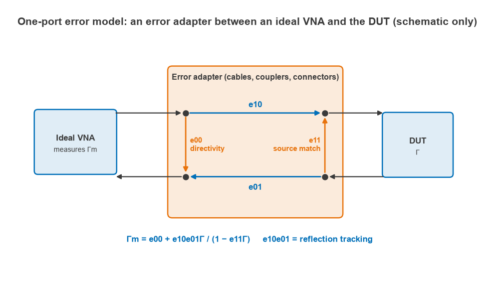
For reflection measurements at one port, the hardware between an ideal reflectometer and the DUT can be represented as a two-port error adapter with three independent terms:
- e00, directivity: signal that reaches the reflected-wave receiver without ever reaching the DUT, mainly coupler leakage and reflections inside the test port.
- e11, source match: the reflection coefficient looking back into the test port from the DUT.
- e10e01, reflection tracking: the combined frequency response of the forward and reverse paths.
The measured reflection Γm relates to the true reflection Γ by:
Γm = e00 + e10e01Γ / (1 − e11Γ)
Three standards with known Γ give three equations for the three unknowns at each frequency point. With an ideal open (Γ = +1), short (Γ = −1) and load (Γ = 0), the solution is compact. The load gives e00 = ML directly. Writing a = MO − e00 and b = MS − e00:
e11 = (a + b)/(a − b), e10e01 = a(1 − e11)
The corrected reflection of any DUT then follows by inverting the model: Γ = (Γm − e00) / (e10e01 + e11(Γm − e00)). Real calibration kits do not have ideal standards, so the analyzer uses a stored definition of each standard: the open’s fringing capacitance polynomial, the short’s inductance, and the offset delay and loss of each.
Worked example: one-port correction
Assume a test port with e00 = 0.0316∠45° (30 dB directivity), e11 = 0.1∠−60° (20 dB source match) and e10e01 = 0.8∠−120°. The raw readings of ideal standards would be:
| Standard | True Γ | Raw measurement Γm |
|---|---|---|
| Open | +1 | 0.8075∠−124.8° |
| Short | −1 | 0.7891∠63.9° |
| Load | 0 | 0.0316∠45.0° |
| DUT | 0.200∠30° (−14.0 dB) | 0.1420∠−81.6° (−17.0 dB) |
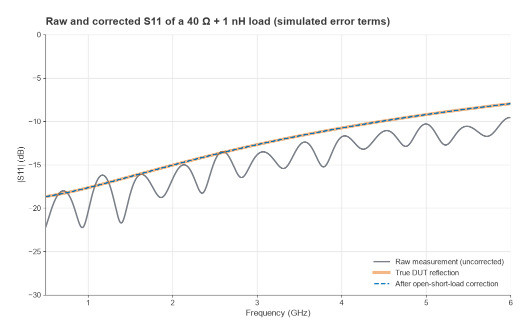
Feeding the three standard readings into the formulas above returns exactly the assumed error terms, and the corrected DUT value comes out as 0.200∠30°. Without correction the DUT reads 3 dB better than it is. Simply dividing the raw magnitude by the tracking magnitude (a response-only calibration) still leaves it at −15.0 dB, a 1 dB error, because directivity and source match are ignored. This is why a full one-port calibration is needed for return loss work, as discussed under VSWR and return loss.
The 12-term two-port error model
A two-port VNA has a forward direction (port 1 driving) and a reverse direction (port 2 driving). Each direction has six error terms, giving twelve in total:
| Forward term | Reverse term | Meaning |
|---|---|---|
| EDF | EDR | Directivity |
| ESF | ESR | Source match |
| ERF | ERR | Reflection tracking |
| ELF | ELR | Load match (the non-driven port seen by the DUT) |
| ETF | ETR | Transmission tracking |
| EXF | EXR | Crosstalk (isolation) |
The reflection terms come from one-port calibrations at each port. A thru connection then yields load match and transmission tracking for each direction, and an optional isolation step with both ports terminated measures crosstalk. Because each corrected S-parameter depends on all four raw S-parameters, the analyzer must measure in both directions before it can correct any one of them. Analyzers with a reference receiver on each port can also use a reduced 8-term model, the basis of TRL and many modern methods, and apply switch-term correction to account for the change in port match when the source switches. The S-parameter definitions are covered on the S-parameters page.
SOLT vs TRL vs ECal
SOLT
SOLT uses a short, open and load at each port and a thru between them. It is the most common coaxial method, works over very wide bandwidths from a single kit, and needs no special fixtures. Its accuracy depends entirely on how well the standards are known. The load is the hardest standard to make perfect at high frequencies, and the thru must be flush (zero length) or precisely defined. SOLT is awkward in non-coaxial media, such as on a PCB, because good open, short and load standards are hard to build there.
TRL
TRL uses a thru, a reflect (any high reflection, the same at both ports, whose phase only needs to be known roughly) and a line of known impedance whose length differs from the thru. The line’s characteristic impedance becomes the reference impedance, so the method does not depend on a precise load. That makes TRL the method of choice in fixtures, on wafer and on PCBs, where a well-made transmission line is easier to build than a broadband 50 Ω termination.
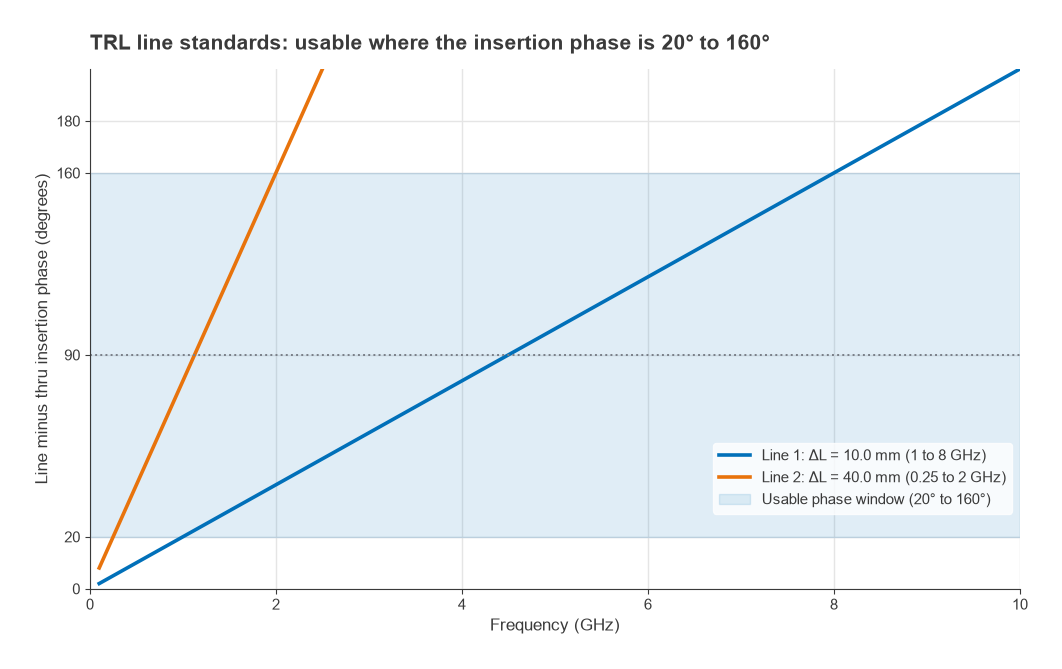
The line’s extra insertion phase must stay clear of 0° and 180°; a common rule keeps it between about 20° and 160°, which covers an 8:1 frequency span. The length is chosen for 90° at the arithmetic centre of the band. For 1 to 8 GHz the centre is 4.5 GHz. On a microstrip with εeff = 2.78, λg = c/(f√εeff) = 40.0 mm at 4.5 GHz, so the line is λg/4 = 10.0 mm longer than the thru. It gives 20° at 1 GHz and 160° at 8 GHz. A second line four times as long (40.0 mm) covers 0.25 to 2 GHz, and below a few hundred megahertz a matched load replaces the line (the TRM variant).
ECal and other automatic methods
Electronic calibration modules contain several switched impedance states that were characterized at the factory against a primary calibration. The analyzer connects once, steps through the states and computes the error terms automatically. ECal is fast, reduces connection wear and removes operator mistakes in choosing standards. Its accuracy is traceable to the module’s own characterization, which ages and is temperature-dependent, so modules need periodic recharacterization. Unknown-thru (SOLR) methods are a related option when the two ports have different connectors or cannot be joined with a flush thru.
| Method | Standards | Best suited to | Main limitation |
|---|---|---|---|
| SOLT | Short, open, load, thru | Coaxial, wide bandwidth | Accuracy set by standard definitions, especially the load |
| TRL | Thru, reflect, line(s) | Fixtures, PCB, on-wafer | Band-limited per line; needs fixtures built for it |
| ECal | Electronic module | Fast, repeatable production work | Depends on module characterization and temperature |
| SOLR | Short, open, load, any reciprocal thru | Non-insertable or mixed-connector setups | Same standard-definition dependence as SOLT |
How to calibrate a VNA: step by step
- Warm up the analyzer for the period its manufacturer recommends, and keep the room temperature stable.
- Set the final frequency range, number of points, IF bandwidth and source power before calibrating. Changing them afterwards can invalidate or interpolate the calibration.
- Fit the cables and adapters that will be used for the measurement and route them as they will lie. Inspect and clean every connector, and use a torque wrench.
- Select the calibration kit definition that matches the physical kit, including the connector gender of each standard.
- Measure each standard as prompted. For SOLT: open, short and load on each port, then the thru, then isolation if required.
- Save the calibration and verify it. A short airline, a known attenuator or a verification kit should read as expected; a load should show return loss consistent with the kit’s specification.
- If the DUT sits in a fixture, move the reference plane to the DUT pins with a fixture calibration (TRL) or with de-embedding.
Port extension is a simpler alternative that removes only the delay, and optionally the loss, of a uniform line between the calibration plane and the DUT. It works well for short, well-matched fixtures but cannot correct mismatches inside the fixture. Calibrated data are usually saved as Touchstone files for simulation, and they can be processed in Python with scikit-rf, which implements the same error models.
Residual errors after calibration
Calibration does not make the analyzer perfect. Imperfect standards leave residual directivity, source match and tracking errors, and these set the measurement uncertainty. Residual directivity matters most when measuring well-matched devices: with 30 dB effective directivity, a DUT with a true return loss of 20 dB can read anywhere between about 17.6 dB and 23.3 dB, and even 40 dB directivity leaves a spread of 19.2 dB to 20.9 dB. Cable flexing and temperature drift add to the residuals over time. The VNA basics page quantifies directivity uncertainty, and measuring radio performance places VNA work within a full test strategy.
Frequently asked questions
How do you calibrate a VNA?
Set the final sweep settings, attach the test cables, choose the matching calibration kit definition, and measure each standard the analyzer prompts for at the cable ends. For a two-port SOLT calibration that means open, short and load on each port, then a thru. Verify the result with a known device before measuring.
What is the difference between SOLT and TRL?
SOLT relies on accurately known short, open, load and thru standards and works over very wide bandwidths in coax. TRL uses a thru, an unknown high reflect and a transmission line whose impedance sets the reference. It suits fixtures and PCBs, but each line covers only about an 8:1 bandwidth.
How often should a VNA be calibrated?
User calibration is repeated whenever the setup changes: different cables, adapters, frequency range or IF bandwidth. It is also repeated when verification shows drift, often at least daily for precise work. The instrument’s own periodic factory calibration is a separate matter.
Related topics
See VNA basics for instrument architecture, de-embedding for fixture removal and noise figure measurement for another calibrated measurement. Spectrum-domain work is covered in spectrum analyzer basics, and the reflection terms used throughout are defined in reflection and transmission coefficients and the wireless terms glossary.