Microstrip Filter Design: Stepped-Impedance, Coupled-Line and Hairpin

Microstrip filter design is the process of building an RF filter from printed transmission-line sections instead of discrete inductors and capacitors. The designer starts from a lumped low-pass prototype, converts its elements into line sections with Richards’ transformation, Kuroda identities or impedance and admittance inverters, picks a layout such as stepped-impedance, parallel coupled-line or hairpin, and then confirms the response with an electromagnetic simulation before building it.

Distributed filters become attractive above roughly 1 to 2 GHz, where lumped parts are small enough for their parasitics to dominate, and where printed lines a fraction of a wavelength long fit on a board. This page works through the three most common microstrip forms with real numbers on a low-loss laminate. It belongs to the RF filters hub of the RF design reference, and it assumes the prototype method covered in LC filter design.

From lumped prototype to distributed filter

Every design on this page starts with normalized low-pass prototype values g₁ to g_N, taken from Butterworth or Chebyshev tables for the required order and ripple. The order and response type come from the specification: passband edge, ripple, and the rejection required at stated offsets, as defined in RF filter specifications. The prototypes used below are:

5th-order Butterworth: g = 0.618, 1.618, 2.000, 1.618, 0.618
3rd-order Chebyshev, 0.5 dB ripple: g = 1.5963, 1.0967, 1.5963, with g₄ = 1.0

The substrate in all examples is a low-loss laminate with ε_r ≈ 3.55 and thickness h = 0.508 mm. Using Hammerstad-type synthesis formulas, a 50 Ω line is 1.14 mm wide with ε_eff = 2.78, a 120 Ω line is 0.17 mm wide (ε_eff = 2.49), and a 20 Ω line is 3.99 mm wide (ε_eff = 3.08). The microstrip calculator gives the same quantities for other stack-ups, and FR4 vs Rogers discusses why filter work favours low-loss materials.

Richards’ transformation and Kuroda identities

Richards’ transformation maps the frequency variable onto Ω = tan(βl). With all lines made λ/8 long at the cutoff frequency f_c, tan(βl) = 1 at f_c, and:

an inductor g_k becomes a short-circuited stub with impedance Z = g_kZ₀
a capacitor g_k becomes an open-circuited stub with impedance Z = Z₀/g_k

Series stubs cannot be built in microstrip, so Kuroda identities are used to convert them into shunt stubs. First, unit elements (λ/8 lines of impedance Z₀) are added at each port; they change only the phase. Then each pair of a unit element and a series stub is swapped for a shunt stub and a new unit element. In one form, checked numerically for this page: a unit element of impedance Z₁ followed by a series short-circuited stub of impedance Z₂ is equivalent to a shunt open-circuited stub of impedance Z₁(Z₁ + Z₂)/Z₂ followed by a unit element of impedance Z₁ + Z₂.

Example: 4 GHz low-pass with stubs

Take the 3rd-order, 0.5 dB Chebyshev prototype in its series-L, shunt-C, series-L form, with f_c = 4 GHz. Richards’ transformation gives series short stubs of 1.5963 × 50 = 79.8 Ω and a shunt open stub of 50/1.0967 = 45.6 Ω. Applying the Kuroda identity at each end with Z₁ = 50 Ω and Z₂ = 79.8 Ω produces:

shunt open stubs of 50 × 129.8/79.8 = 81.3 Ω at each port (0.47 mm wide, 5.79 mm long)
unit elements of 129.8 Ω between the stubs (0.13 mm wide, 5.97 mm long)
the centre shunt open stub of 45.6 Ω (1.31 mm wide, 5.59 mm long)

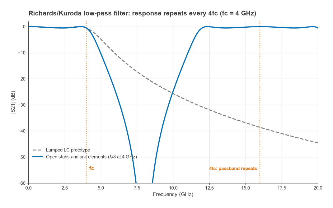
The computed response matches the prototype exactly at 4 GHz (0.50 dB ripple) and rolls off faster above it, because tan(βl) grows faster than frequency. The price is periodicity. At 8 GHz the stubs are λ/4 long and present short circuits, giving a deep notch, and at 16 GHz (4f_c) the lines are λ/2 long and the passband returns in full. The 129.8 Ω unit element is also close to the narrowest trace many board shops produce reliably on this substrate, a common limitation of Kuroda designs.

S21 of a 4 GHz stub low-pass filter versus its LC prototype, showing a notch at 8 GHz and passband repeating at 16 GHz — Figure 1: Computed response of the 3rd-order, 0.5 dB Chebyshev stub filter (81.3 Ω and 45.6 Ω stubs, 129.8 Ω unit elements). The passband returns at 4fc = 16 GHz.

Stepped-impedance low-pass filters

A short line of high impedance Z_h behaves approximately like a series inductor, and a short line of low impedance Z_l like a shunt capacitor. For a prototype normalized to Z₀, the electrical lengths at f_c are:

βl = g_kZ₀/Z_h for an inductor, and βl = g_kZ_l/Z₀ for a capacitor

The approximation holds best when βl is well below 45° and the impedance ratio Z_h/Z_l is as large as the process allows.

Worked example: 2.5 GHz stepped-impedance filter

Using the 5th-order Butterworth prototype in shunt-C-first form, f_c = 2.5 GHz, Z_h = 120 Ω and Z_l = 20 Ω:

Section	Prototype g	Line	βl at 2.5 GHz	Width	Length
1 (C)	0.618	20 Ω	14.2°	3.99 mm	2.69 mm
2 (L)	1.618	120 Ω	38.6°	0.17 mm	8.16 mm
3 (C)	2.000	20 Ω	45.8°	3.99 mm	8.70 mm
4 (L)	1.618	120 Ω	38.6°	0.17 mm	8.16 mm
5 (C)	0.618	20 Ω	14.2°	3.99 mm	2.69 mm

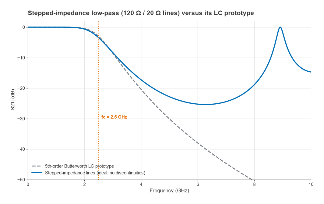
Lengths use λ_g = c/(f√ε_eff) for each line. Cascading the ideal line sections gives 3.5 dB of loss at 2.5 GHz instead of the prototype’s 3.0 dB, 17.3 dB of rejection at 4 GHz (prototype 20.5 dB) and 22.8 dB at 5 GHz (prototype 30.1 dB). Rejection then degrades, and the line filter has a spurious passband near 8.9 GHz. Stepped-impedance filters are compact and simple, but they suit applications that need only moderate stopband rejection, such as harmonic clean-up after an oscillator.

S21 of a 5th-order stepped-impedance low-pass filter compared with its Butterworth prototype up to 10 GHz — Figure 2: Ideal 120 Ω / 20 Ω line sections track the prototype to about 3 GHz, then rejection levels off near 23 dB and a spurious passband appears near 8.9 GHz.

Coupled-line bandpass filter design flow

A parallel coupled-line filter uses half-wave resonators that couple to each other over quarter-wave overlaps. Each coupled section acts as an admittance inverter J plus line lengths, so the low-pass prototype maps directly onto even- and odd-mode impedances. For fractional bandwidth Δ and N resonators:

Z₀J₁ = √(πΔ/(2g₀g₁))
Z₀J_n = πΔ/(2√(g_n−1g_n)), for n = 2 to N
Z₀J_N+1 = √(πΔ/(2g_Ng_N+1))
Z_0e = Z₀[1 + JZ₀ + (JZ₀)²], Z_0o = Z₀[1 − JZ₀ + (JZ₀)²]

Worked example: 2.45 GHz, 10% bandwidth

Specification: centre 2.45 GHz, Δ = 0.10, 0.5 dB ripple, at least 20 dB rejection at 2.2 and 2.7 GHz. A 3rd-order Chebyshev prototype is chosen.
Inverters: Z₀J₁ = Z₀J₄ = 0.3137 and Z₀J₂ = Z₀J₃ = 0.1187.
Mode impedances: sections 1 and 4 need Z_0e = 70.6 Ω and Z_0o = 39.2 Ω; sections 2 and 3 need Z_0e = 56.6 Ω and Z_0o = 44.8 Ω.
Geometry: a coupled-line synthesis tool or a 2D field solver converts each pair into strip width and gap. The end sections need the tightest gap, which usually sets the minimum feature size.
Lengths: each section is a quarter of the guided wavelength at f₀, about 18 mm on this substrate before correction for even- and odd-mode velocity differences and open-end fringing.

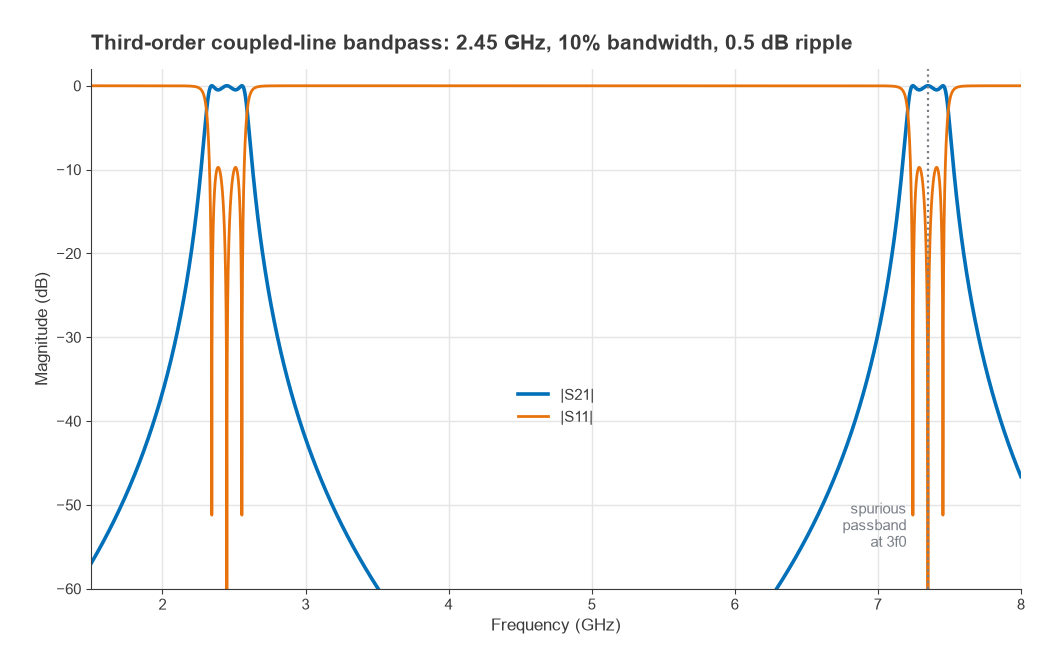
The ideal coupled-line model gives a 3 dB bandwidth of 2.308 to 2.592 GHz, passband ripple within 0.5 dB, and exactly 20.0 dB of rejection at 2.2 and 2.7 GHz, rising to 36.6 dB at 2.0 GHz and 42.1 dB at 3.0 GHz. Like every half-wave resonator filter, it has a spurious passband at 3f₀, here 7.35 GHz. In microstrip, unequal even- and odd-mode phase velocities also create a weaker spurious response near 2f₀, which is one reason EM verification is needed.

S21 and S11 of a third-order coupled-line bandpass filter at 2.45 GHz with spurious passband at 7.35 GHz — Figure 3: Ideal coupled-line model with Z0e/Z0o of 70.6/39.2 Ω and 56.6/44.8 Ω. The 3 dB band is 2.308 to 2.592 GHz; a spurious passband appears at 3f0.

Hairpin filters

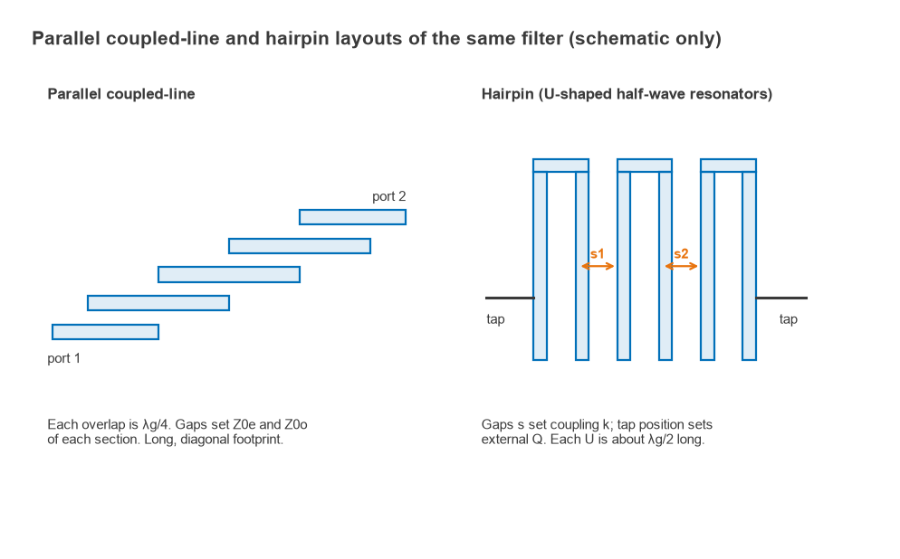
A parallel coupled-line filter is long and diagonal. Folding each half-wave resonator into a U shape gives a hairpin filter with the same electrical design and a much more compact, rectangular footprint. Hairpin designs are usually set up with coupling coefficients and external Q, which can be extracted from EM simulations of resonator pairs:

k_i,i+1 = Δ/√(g_ig_i+1), Q_e = g₀g₁/Δ

For the same 3rd-order, 10% design, k₁₂ = k₂₃ = 0.0756 and Q_e = 16.0. The flow is:

Simulate one U resonator and adjust its total length (about λ_g/2) to resonate at 2.45 GHz. Keep the two arms far enough apart that they do not couple strongly to each other.
Simulate two weakly excited resonators at gap s. The two resonant peaks f₁ and f₂ give k = (f₂² − f₁²)/(f₂² + f₁²). Sweep s and read off the gap for k = 0.0756.
Simulate one resonator with a tapped 50 Ω feed. The loaded Q from the 3 dB bandwidth of the group delay or reflection response gives Q_e. Move the tap until Q_e = 16.0.
Assemble the full filter and run a complete EM simulation, then fine-tune lengths for centre frequency and gaps for bandwidth.

Layout sketches of a parallel coupled-line filter and a three-resonator hairpin filter with tapped feeds — Figure 4: Schematic only, not to scale. Both layouts implement the same coupling; the hairpin folds each half-wave resonator to shorten the footprint.

EM verification and fabrication effects

The closed-form results above ignore open-end fringing, step discontinuities between wide and narrow lines, T-junction parasitics, dispersion, conductor and dielectric loss, radiation, and enclosure resonances. A planar EM solver (method of moments) captures most of these for a microstrip filter, and a 3D solver is needed if the filter sits under a shield or near other structures. EM simulation basics and RF simulation software cover the tools.

Simulate with the actual copper thickness, surface roughness and loss tangent of the laminate.
Run a tolerance analysis on etch width (often a few tens of micrometres) and ε_r; narrow-band filters are the most sensitive.
Include the shield lid if one is used, since it lowers ε_eff differently for even and odd modes and can add box resonances.
Measure the built filter on a calibrated VNA with good fixtures, as described in VNA calibration and VNA basics.

Insertion loss rises roughly in proportion to the number of resonators and inversely with fractional bandwidth and resonator Q. Microstrip resonators have modest unloaded Q, so narrow filters of a few percent bandwidth often move to stripline, cavity or acoustic technologies, compared in SAW vs BAW filters.

Frequently asked questions

How do you design a microstrip bandpass filter?

Choose a Chebyshev or Butterworth prototype that meets the ripple and rejection specification, then convert it into inverter values for the chosen fractional bandwidth. Compute the even- and odd-mode impedances for a coupled-line filter, or coupling coefficients and external Q for a hairpin, turn them into widths and gaps, and verify the complete layout in an EM simulator.

Why does a microstrip filter have spurious passbands?

Transmission lines repeat their behaviour every half wavelength, so a filter built from them repeats its response. Half-wave resonator filters show a passband again near 3f₀, and microstrip’s unequal mode velocities can add a response near 2f₀. A low-pass filter in cascade, or stepped-impedance resonators, push these responses away.

When should I use a hairpin instead of a coupled-line filter?

Use a hairpin when board area matters. It has the same electrical design but folds each resonator, so the footprint is much shorter. The coupled-line form is easier to design from closed-form equations and is common in teaching and quick prototypes.