

Commercial RF simulation software falls into two classes: circuit simulators with planar EM, such as Keysight ADS and Cadence Microwave Office, and full-wave 3D field solvers, such as Ansys HFSS, Dassault Systèmes CST Studio Suite and the planar specialist Sonnet. ADS and Microwave Office cover similar ground, with harmonic balance, layout and 2.5D EM; the choice between them usually comes down to existing design flows, process design kits and team familiarity rather than solver capability.
No single tool does everything equally well. A complete RF design normally passes through circuit simulation for gain, noise and linearity, an electromagnetic (EM) solve of the layout or enclosure, and then co-simulation of the EM results with active devices. This page compares the five most widely used commercial packages by solver type, typical use and licensing model, explains the numerical methods behind them, and gives rules for picking a tool for a given problem. It is part of the RF engineering tools and resources section of the RF design reference. Prices are not given here: they are quoted per customer, depend on modules and term, and change frequently.
Circuit simulators and EM solvers
A circuit simulator works with lumped and distributed models connected at nodes. Linear analysis gives S-parameters and noise; harmonic balance solves nonlinear steady-state problems such as compression, intermodulation and mixer conversion in the frequency domain; transient and envelope analysis handle modulated signals and start-up. Circuit simulation is fast, but its accuracy depends on how well the models describe the real layout. The method is covered in harmonic balance simulation.
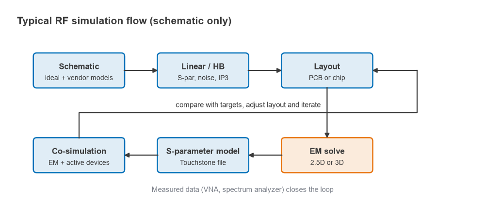
An EM solver starts from geometry and materials and solves Maxwell’s equations directly. It captures coupling, radiation, package and enclosure effects and discontinuities that circuit models miss, and it produces S-parameters that can be returned to the circuit simulator as a Touchstone file. The principal methods are:
- Method of moments (MoM), 2.5D planar. Solves for currents on metal layers in a stratified dielectric stack. Very efficient for PCB and MMIC traces, filters and planar antennas, but it assumes laterally infinite or box-enclosed layers and cannot represent arbitrary 3D objects.
- Finite element method (FEM), 3D frequency domain. Meshes the whole volume with tetrahedra and solves at each frequency. It handles arbitrary 3D shapes, connectors, packages, waveguides and resonant structures well, with adaptive mesh refinement.
- Time-domain methods (FIT, FDTD). March the fields forward in time on a grid. One run with a broadband pulse gives the response over a wide band, which suits electrically large, broadband and transient problems such as antennas in housings, EMC and signal integrity.
- Integral equation and asymptotic methods. Used for electrically very large problems, such as antennas on vehicles or radar cross section, where volume meshing would be impractical.
A fuller introduction to meshing, ports and boundaries is in EM simulation basics.
The five main commercial tools
Keysight ADS
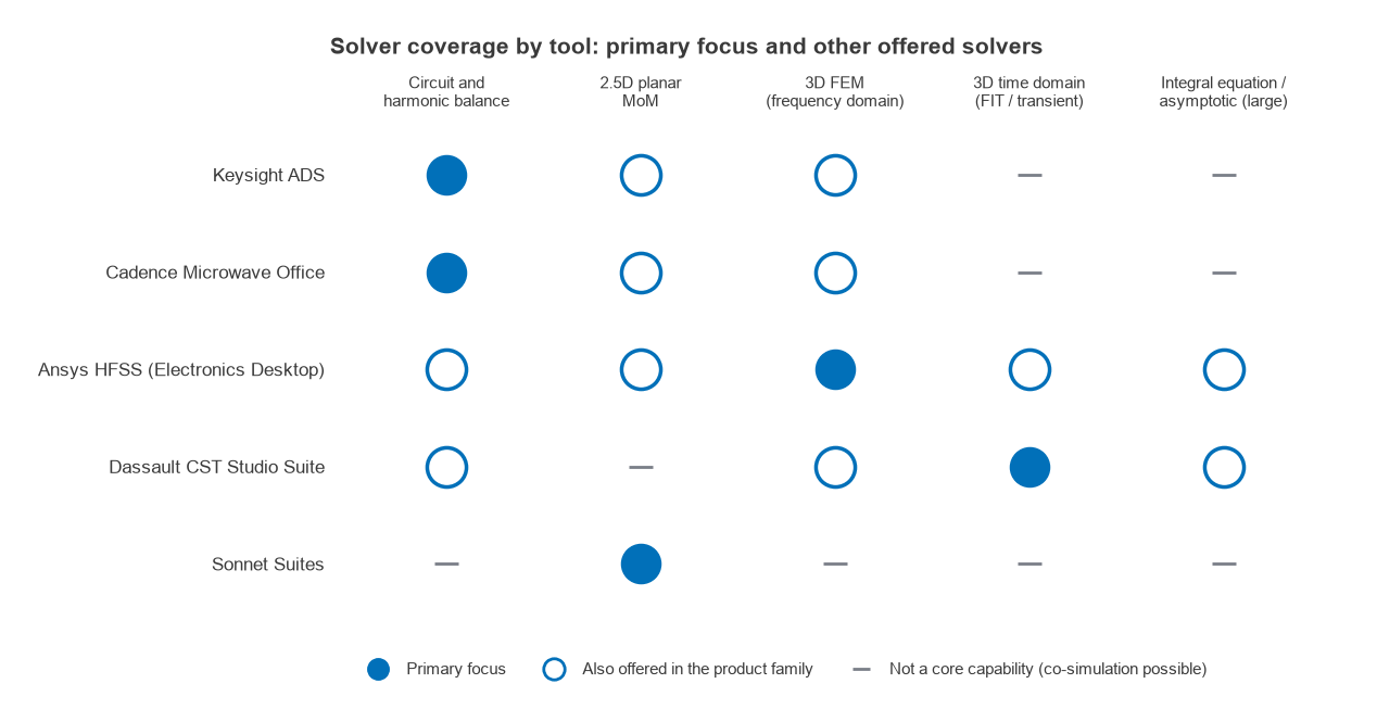
Keysight Advanced Design System is a circuit and system design environment with linear, harmonic balance, transient, envelope and X-parameter analysis, and integrated layout. Momentum provides 2.5D MoM, and 3D FEM is available within the same environment. ADS is widely used for power amplifier design, MMIC and module work, and has broad support from foundry process design kits and device vendor models.
Cadence Microwave Office
Cadence Microwave Office, originally from AWR, covers similar ground: linear and harmonic balance circuit simulation, layout, the AXIEM 2.5D MoM solver and the Analyst 3D FEM solver. It is known for interactive tuning and a quick path from schematic to layout, and it links to the wider Cadence IC and PCB flows. ADS vs Microwave Office is therefore mostly a question of ecosystem: which PDKs the foundry supports, which tool the team and its customers already use, and how it connects to the rest of the design flow.
Ansys HFSS
Ansys HFSS is a 3D FEM solver with adaptive meshing, widely used for antennas, connectors, packages, waveguide components and anything where 3D field accuracy matters. Within the Electronics Desktop environment it is joined by integral equation, transient and asymptotic solvers and by circuit simulation for co-simulation.
Dassault Systèmes CST Studio Suite
Dassault Systèmes CST Studio Suite is best known for its time-domain finite integration technique (FIT) solver, with frequency-domain FEM, integral equation and asymptotic solvers in the same package, and a schematic environment for system and circuit co-simulation. It is common in antenna, EMC and signal integrity work and for electrically large, broadband structures.
Sonnet
Sonnet is a specialist 2.5D planar MoM solver for structures in a shielded box. It is valued for accuracy on planar circuits, including thin-film, superconducting and high-Q filter work, and it can be used from within other design environments. A limited free version has been offered for learning and small problems.
Comparison table: solver types, use cases, licensing
The summary reflects each product family’s general positioning as of 2026. Module names and bundles change, so confirm current capabilities with the vendor.
| Tool | Core solvers | Strongest use cases | Licensing model |
|---|---|---|---|
| Keysight ADS | Linear, harmonic balance, transient, envelope; 2.5D MoM (Momentum); 3D FEM | PA and MMIC design, modules, system-level RF and co-simulation | Commercial, modular bundles; time-based or perpetual with maintenance; node-locked or floating; university programs |
| Cadence Microwave Office | Linear, harmonic balance; 2.5D MoM (AXIEM); 3D FEM (Analyst) | MMIC, PCB RF and module design with interactive tuning | Commercial, modular; time-based or perpetual; node-locked or floating; university programs |
| Ansys HFSS | 3D FEM; integral equation, transient and asymptotic solvers in the same environment | Antennas, connectors, packages, waveguide and 3D passive components | Commercial, typically time-based leases or perpetual; capacity-based options for HPC; free student edition with size limits |
| Dassault CST Studio Suite | 3D time-domain FIT; frequency-domain FEM; integral equation; asymptotic | Broadband antennas, antennas in housings, EMC, signal integrity | Commercial, modular; token or feature based; free student edition with size limits |
| Sonnet | 2.5D shielded planar MoM | High-accuracy planar circuits and filters, thin-film and superconducting circuits | Commercial tiers by feature and problem size; limited free version |
Computational cost: worked examples
Understanding how each method scales helps decide where to use it. Three short calculations show the main limits.
MoM: memory grows as N squared
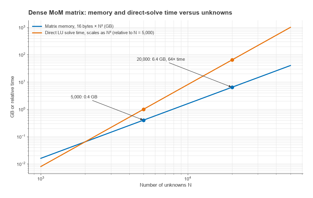
A classic MoM solver fills a dense N × N matrix of complex double-precision values, 16 bytes each. At N = 5,000 unknowns, the matrix needs 16 × 5,0002 = 0.4 GB. At N = 20,000 it needs 6.4 GB, and a direct LU solve, whose time scales as N3, takes (20,000/5,000)3 = 64 times longer. Refining the mesh by a factor of two in each planar direction roughly quadruples N, so mesh density on large planar layouts must be chosen with care. Modern solvers use compression and iterative methods to soften this scaling, but the trend is why 2.5D tools work best on circuits a few wavelengths across.
Time domain: the Courant limit
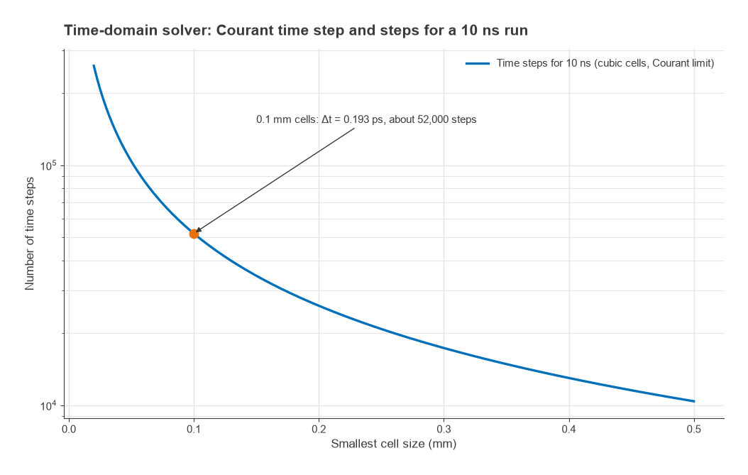
An explicit time-domain solver must keep its time step below the Courant limit. For cubic cells of side Δ in free space,
Δt ≤ Δ / (c√3)
With 0.1 mm cells, needed to resolve a fine trace gap, Δt = 0.1 mm / (3.0 × 10⁸ m/s × 1.732) = 0.193 ps, so a 10 ns run needs about 51,900 time steps. Halving the smallest cell to 0.05 mm doubles the step count to about 104,000, as well as multiplying the number of cells. A 50 × 50 × 10 mm region meshed uniformly at 0.1 mm already contains 25 million cells, which is why time-domain tools use non-uniform meshes and subgridding. The advantage is that one run covers the whole band.
FEM: elements per wavelength
FEM meshes need several elements per wavelength in each material. At 10 GHz in a substrate with εr = 3.5, the wavelength is 30 mm / √3.5 = 16.0 mm, so a common starting rule of about λ/10 gives 1.6 mm maximum element size in the dielectric, with much finer elements near conductor edges. Adaptive refinement does this automatically, but the volume of a large enclosure or a long cable still makes 3D FEM expensive, and the cost repeats at each frequency point unless a fast sweep is used.
Which tool for which job
- Amplifiers, mixers and oscillators: a circuit simulator with harmonic balance and good device models, ADS or Microwave Office, with planar EM for the layout.
- Planar filters and matching networks: 2.5D MoM (Momentum, AXIEM or Sonnet), which is fast and accurate for layered structures. See microstrip filter design.
- Connectors, packages, transitions and waveguides: 3D FEM, typically HFSS, or the FEM solvers in the other suites.
- Antennas in real products, EMC and broadband transients: 3D time-domain (CST) or 3D FEM with a full model of the housing.
For PCB antennas specifically, a 2.5D solver is adequate for early sizing when the board is large compared with the antenna and nothing else is nearby. Once the finite ground plane, the plastic housing, the battery and the feed cable matter, which is almost always the case in a final product, a 3D FEM or time-domain solver is the safer choice. The antenna side of this is covered in PCB antenna design.
Commercial tools are not the only route. Open-source and free options, along with Python packages for processing S-parameters, are compared in free RF design software and Python and scikit-rf for RF engineers, and quick hand calculations are collected in RF calculators.
Frequently asked questions
ADS vs Microwave Office: which is better?
Both offer linear and harmonic balance circuit simulation, layout, 2.5D MoM and 3D FEM. The practical difference is the ecosystem: foundry PDK support, device model libraries, links to IC and PCB tools, and what colleagues and customers use. Many engineers evaluate both on a real design during a trial before committing.
Which EM simulator is best for PCB antennas?
For early sizing on a large ground plane, a 2.5D planar solver is fast and adequate. For the final design, where the finite board, housing, nearby components and cable affect tuning and efficiency, a 3D solver such as an FEM or time-domain tool gives more trustworthy results.
What is the difference between 2.5D and 3D EM simulation?
A 2.5D solver models flat metal layers in a layered dielectric stack and solves only for surface currents, which makes it fast for PCB and chip interconnect. A 3D solver meshes the full volume and can model arbitrary shapes, such as connectors, enclosures and bond wires, at higher computational cost.
Are there free versions of commercial RF simulators?
Some vendors offer free student or limited editions with restrictions on problem size, and most run university programs and time-limited trials. Terms change, so check each vendor’s site for current offers.
Related topics
Simulated S-parameters are best checked against measurement, as described in VNA basics, and antenna results against antenna parameters measured in a chamber. The wider set of tools and learning resources is gathered in RF engineering tools and resources, and terms are defined in the wireless terms glossary.