SAW vs BAW Filters: Frequency, Q, TCF and Power Compared

SAW and BAW filters are both acoustic resonator filters, and the difference between them is where the acoustic wave travels. A surface acoustic wave (SAW) filter launches a wave along the surface of a piezoelectric crystal and works best below about 2.5 GHz. A bulk acoustic wave (BAW) filter sets up a wave through the thickness of a thin piezoelectric film. It reaches higher frequencies, typically up to 6 GHz and beyond, with higher Q, but it costs more.

Acoustic filters are used where an LC or microstrip filter would be far too large or too lossy for the selectivity required, mainly in handset and IoT front ends. An acoustic wave moves about five orders of magnitude more slowly than an electromagnetic wave, so a resonator a few micrometres across can resonate at gigahertz frequencies, and its Q is far higher than a lumped LC tank of similar size. This page compares the two technologies on frequency range, Q, temperature coefficient, power handling and cost, with worked numbers for each. It belongs to the RF filters section of the RF design reference.

How SAW and BAW resonators work

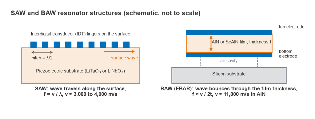
Schematic cross-sections of a SAW resonator with IDT fingers and an FBAR BAW resonator with AlN film over an air cavity — Figure 1: SAW and BAW resonator structures (schematic only, not to scale). SAW frequency is set by finger pitch, BAW frequency by film thickness.

SAW: interdigital transducers on a crystal

A SAW resonator is a pattern of interleaved metal fingers, the interdigital transducer (IDT), deposited on a piezoelectric substrate such as lithium tantalate (LiTaO₃) or lithium niobate (LiNbO₃). An RF voltage between alternate fingers launches a surface wave, and reflector gratings on each side trap it to form a resonant cavity. The finger pitch is half the acoustic wavelength, so the resonant frequency is

f = v / λ = v / (2p)

where v is the surface wave velocity, typically 3,000 to 4,000 m/s, and p is the finger pitch. With v = 3,900 m/s, a 2 GHz resonator needs λ = 1.95 µm, and each finger, at a quarter wavelength, is only 0.49 µm wide. At 3.5 GHz the finger width falls to 0.28 µm. Such narrow fingers are harder to pattern, carry more resistive loss and are more easily damaged at high power. That scaling is the main reason conventional SAW filters are uncommon above about 2.5 to 3 GHz.

BAW: a thin film between two electrodes

A BAW resonator is a thin piezoelectric film, usually aluminium nitride (AlN) or scandium-doped AlN (ScAlN), sandwiched between two electrodes. The wave travels up and down through the film, and resonance occurs when the thickness t is about half an acoustic wavelength:

f ≈ v / (2t)

The longitudinal velocity in AlN is about 11,000 m/s, so a 2 GHz resonator needs a film roughly 2.75 µm thick, and 5.5 GHz needs about 1.0 µm, before allowing for electrode mass, which lowers the required thickness further. Frequency is set by a deposited film thickness rather than by lithography, so BAW scales upward much more easily than SAW. The resonator must be acoustically isolated from the substrate, either with an air cavity underneath (the film bulk acoustic resonator, FBAR) or with a Bragg reflector stack of alternating high and low impedance layers (the solidly mounted resonator, SMR).

Resonator model, coupling and Q

Both resonators are described electrically by the Butterworth-Van Dyke (BVD) model: a static capacitance C₀ in parallel with a series motional branch L_m, C_m, R_m. The motional branch gives a series resonance f_s, where impedance is very low, and the combination with C₀ gives a parallel resonance f_p slightly higher, where impedance is very high. The spacing between them is set by the effective electromechanical coupling coefficient:

k²_eff = (π²/4) × (f_p − f_s) / f_p

For AlN BAW, k²_eff is typically about 6 to 7 %. At f_s = 2 GHz and k²_eff = 6.5 %, the parallel resonance lands at 2054 MHz, a spacing of 54 MHz. In a ladder filter, series resonators and shunt resonators are offset so that the shunt f_p and series f_s align at the centre of the passband. The achievable bandwidth is therefore limited to roughly the resonator spacing, a few percent of the centre frequency. ScAlN raises the coupling and so the bandwidth.

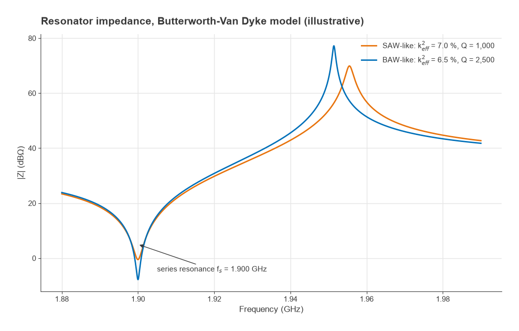
Butterworth-Van Dyke impedance of SAW-like and BAW-like resonators with series resonance at 1.900 GHz — Figure 2: BVD-model impedance with fs = 1.900 GHz. The BAW-like resonator (Q = 2,500) has a deeper minimum and higher peak than the SAW-like one (Q = 1,000). Illustrative values.

The quality factor sets the loss and the sharpness of the skirts. Published BAW resonators commonly reach unloaded Q values of about 1,500 to 4,000 near 2 GHz. Conventional SAW resonators are typically lower, often in the range of about 500 to 1,500, although newer multilayer SAW structures close much of the gap. See Q factor in RF circuits for the general definition.

Worked example: insertion loss from resonator Q

A first estimate of midband insertion loss for a filter built from resonators of unloaded Q_u is Cohn’s formula:

IL ≈ 4.343 × (f₀ / BW) × Σg_k / Q_u (dB)

where g_k are the lowpass prototype values. For a fifth-order Chebyshev response with 0.1 dB ripple, Σg_k = 1.1468 + 1.3712 + 1.9750 + 1.3712 + 1.1468 = 7.011. Take f₀ = 2 GHz and BW = 60 MHz, so f₀/BW = 33.3.

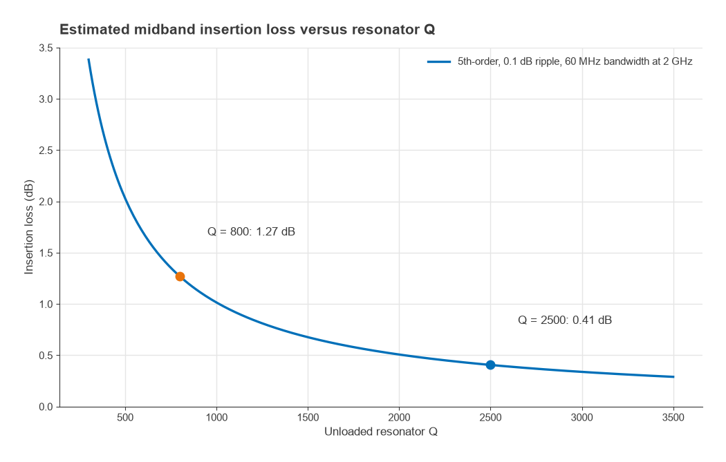
Estimated insertion loss versus resonator Q for a 60 MHz wide filter at 2 GHz, 1.27 dB at Q 800 and 0.41 dB at Q 2500 — Figure 4: Cohn estimate for a fifth-order, 0.1 dB ripple, 60 MHz filter at 2 GHz: 1.27 dB at Qu = 800 and 0.41 dB at Qu = 2,500.

With Q_u = 800, typical of a SAW resonator: IL ≈ 4.343 × 33.3 × 7.011 / 800 = 1.27 dB.
With Q_u = 2,500, typical of a BAW resonator: IL ≈ 0.41 dB.

Acoustic ladder filters are not classical coupled-resonator filters, so the formula is a guide to scale rather than a prediction. It still shows the trend clearly: loss is inversely proportional to Q and to fractional bandwidth. Close to 0.9 dB of extra loss in a receive path adds almost directly to the receiver’s noise figure, and in a transmit path it costs PA output power and battery life.

Temperature coefficient of frequency

Acoustic velocity changes with temperature, so the whole filter response slides in frequency. The temperature coefficient of frequency (TCF) is given in ppm/K, and the shift is

Δf = TCF × f × ΔT

Common LiTaO₃ SAW cuts have a TCF of roughly −35 to −45 ppm/K. AlN BAW is typically around −25 to −30 ppm/K. Temperature-compensated SAW (TC-SAW) adds a silicon dioxide overlay, whose velocity rises with temperature, and brings the TCF down to roughly −10 to −20 ppm/K. Oxide compensation layers are also used in BAW stacks.

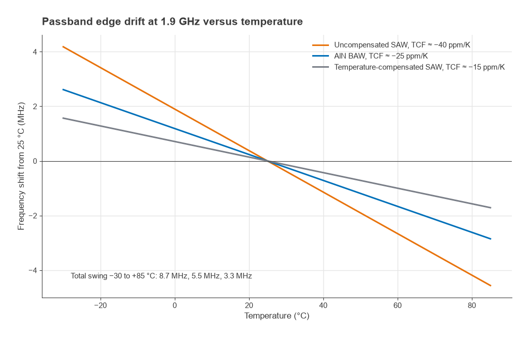
Frequency shift of a 1.9 GHz filter edge versus temperature for TCF of -40, -25 and -15 ppm/K — Figure 3: Edge drift at 1.9 GHz from −30 to +85 °C: 8.7 MHz at −40 ppm/K, 5.5 MHz at −25 ppm/K and 3.3 MHz at −15 ppm/K.

Consider a filter edge at 1.9 GHz over −30 °C to +85 °C, a span of 115 K. At −40 ppm/K the edge moves 40 × 10⁻⁶ × 1.9 × 10⁹ × 115 = 8.7 MHz. At −25 ppm/K it moves 5.5 MHz, and at −15 ppm/K it moves 3.3 MHz. If the transmit and receive bands of a duplexer are separated by a 20 MHz gap, an uncompensated SAW design spends almost half that gap on temperature drift alone, before manufacturing tolerance, and the remaining transition must be achieved with steeper skirts, which means more resonators and more loss. This is why narrow-gap bands are a natural home for BAW or TC-SAW, and why the guard bands in the filter specification must include drift.

Power handling and linearity

Transmit filters and duplexers sit after the power amplifier, so they must carry roughly +30 dBm in handset applications without drifting or degrading. In a SAW device the acoustic energy is concentrated in a thin surface layer under narrow fingers. High stress causes acoustomigration of the finger metal over time, and the heat must leave through a substrate of modest thermal conductivity. BAW resonators spread the energy through the film volume, have no fine fingers, and sit on silicon, which conducts heat better. BAW therefore generally has more power margin at a given frequency, especially above 2 GHz.

Both technologies generate small nonlinear products, particularly second and third harmonics and intermodulation between transmit signals and blockers. In carrier aggregation and multi-radio designs those products can fall into a receive band, so filter linearity is specified as well as loss. The mechanisms are covered under harmonic distortion and receiver blocking and desensitization.

SAW vs BAW comparison table

The figures below are typical approximate ranges as of 2026, gathered from general published behaviour of each technology rather than from any one vendor. Individual products vary widely.

Property	SAW	TC-SAW	BAW (FBAR or SMR)
Practical frequency range	Tens of MHz to about 2.5 GHz	About 0.6 to 2.7 GHz	About 1.5 GHz to 6 GHz and above
Unloaded Q near 2 GHz	About 500 to 1,500	About 800 to 1,500	About 1,500 to 4,000
TCF	About −35 to −45 ppm/K	About −10 to −20 ppm/K	About −25 to −30 ppm/K uncompensated, lower with oxide layers
Frequency set by	Lithographic finger pitch	Pitch plus oxide thickness	Film and electrode thickness
Power handling	Moderate, limited by finger stress and heat	Moderate	Higher, better heat path
Relative cost	Lowest	Medium	Highest
Typical uses	Sub-2 GHz receive filters, IF filters, GNSS, IoT	Cellular duplexers with tight gaps below 2.7 GHz	Bands above 2 GHz, narrow-gap duplexers, Wi-Fi coexistence filters

Choosing between SAW and BAW

The choice usually follows from three questions.

What is the frequency? Below about 1.5 GHz, SAW is normally the cheaper and adequate choice. Above about 2.5 GHz, BAW or a newer multilayer SAW structure is usually required.
How close is the nearest band to be rejected? A narrow transition calls for high Q and low TCF, which favour BAW or TC-SAW.
How much power passes through it? A receive-only filter after the antenna switch sees little power. A transmit filter or duplexer next to the PA needs the larger power margin of BAW, particularly at higher frequencies.

When the bandwidth is very wide, for example a fractional bandwidth well above the acoustic coupling limit, neither technology suits, and an LC filter or a ceramic or microstrip design is used instead. The options are described in LC filter design and microstrip filter design. Acoustic filters are most often bought as part of an integrated module; how they combine with switches and amplifiers is covered in RF front-end modules, and the duplexing function itself in duplexer vs diplexer.

Frequently asked questions

What is the difference between SAW and BAW filters?

A SAW filter uses a wave travelling along the surface of a piezoelectric crystal, with frequency set by the spacing of metal fingers. A BAW filter uses a wave travelling through the thickness of a thin film, with frequency set by film thickness. BAW reaches higher frequencies with higher Q and better power handling, while SAW is cheaper and dominant below about 2 GHz.

Why can’t SAW filters go to high frequencies?

The finger width is a quarter of the acoustic wavelength, so it shrinks in proportion to 1/f. At 3.5 GHz a typical SAW finger is under 0.3 µm wide, which raises resistive loss, makes manufacture harder and lowers power handling. BAW avoids this because thickness, not lateral pitch, sets the frequency.

What is TC-SAW?

TC-SAW is a temperature-compensated SAW filter with a silicon dioxide layer over the transducer. The oxide’s velocity changes with temperature in the opposite direction to the substrate’s, cutting the temperature coefficient from roughly −40 ppm/K to roughly −15 ppm/K, which allows narrower guard bands.

What is the difference between FBAR and SMR?

Both are BAW resonators. An FBAR suspends the piezoelectric film over an air cavity, while an SMR sits on a Bragg reflector of alternating acoustic layers that reflects the wave back into the film. FBARs tend to reach slightly higher Q; SMRs are mechanically sturdier and conduct heat to the substrate more directly.