

Stripline is a planar transmission line in which a flat conductor is buried in a uniform dielectric between two parallel ground planes. Because the field sits entirely inside one material, it carries a pure TEM wave with no dispersion and almost no radiation. Use stripline when isolation, shielding and stable phase matter more than easy access to the trace, typically on inner layers of a multilayer board.
Stripline gives up the surface access of microstrip in exchange for a closed, predictable field. This page covers the symmetric and offset stripline equations, how propagation in a homogeneous dielectric differs from microstrip, the main loss terms, and a full 50 Ω design worked through on a common laminate. It sits within the transmission line theory section of the RF design guide.
Stripline Geometry
Four quantities matter: the strip width W, the strip thickness t, the ground-plane spacing b and the relative permittivity εr of the filling. In symmetric (centred) stripline the strip sits halfway between the planes, so b = 2h + t, where h is the dielectric height above and below the strip. In offset or asymmetric stripline the strip is closer to one plane, with heights h1 and h2. Offset stripline is common because stack-ups mix cores and prepregs of different thickness, and because dual stripline places two signal layers between one pair of planes.
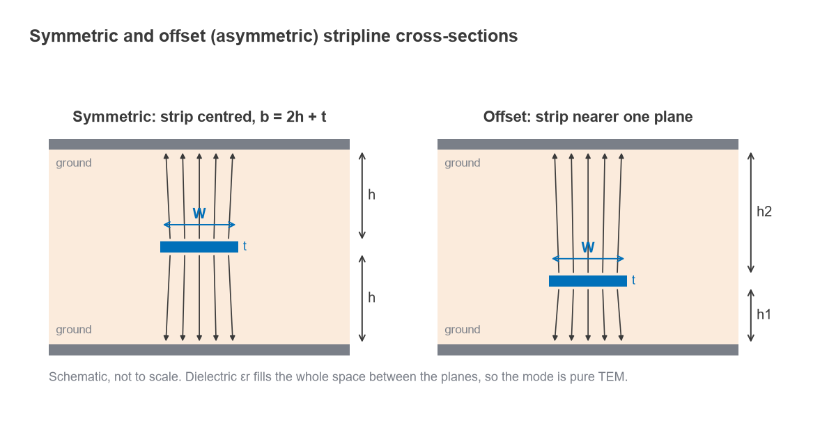
The two ground planes must be at the same potential. If they are not tied together at regular intervals, the pair can carry a parallel-plate mode that couples energy between unrelated lines. Rows of ground vias, often called a via fence, run along both sides of the line for this reason. The general comparison with other line types is in characteristics and types of transmission lines.
TEM Propagation and No Dispersion
Because the dielectric is homogeneous, the wave travels as a true TEM mode. The phase velocity and propagation constant follow directly from the material:
vp = c/√εr, β = ω√εr/c, εeff = εr
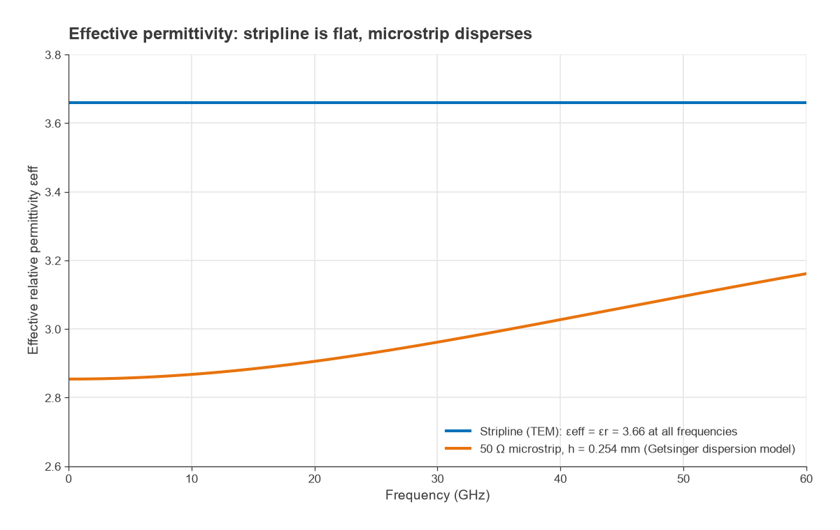
The effective permittivity equals the material permittivity and does not change with frequency or width. In microstrip, part of the field is in air, so εeff lies between 1 and εr and rises with frequency as the field is pulled into the substrate. That dispersion distorts wideband signals and shifts resonator lengths. A stripline delay line keeps the same electrical length ratio across the band, which simplifies the wave propagation analysis. Strictly, the material’s own εr varies slightly with frequency, but that is not caused by the line geometry. The closed structure also means the line itself does not radiate; radiation and coupling occur only at vias, layer transitions and gaps in the ground planes.
Symmetric Stripline Impedance Formulas
Exact result for a thin strip
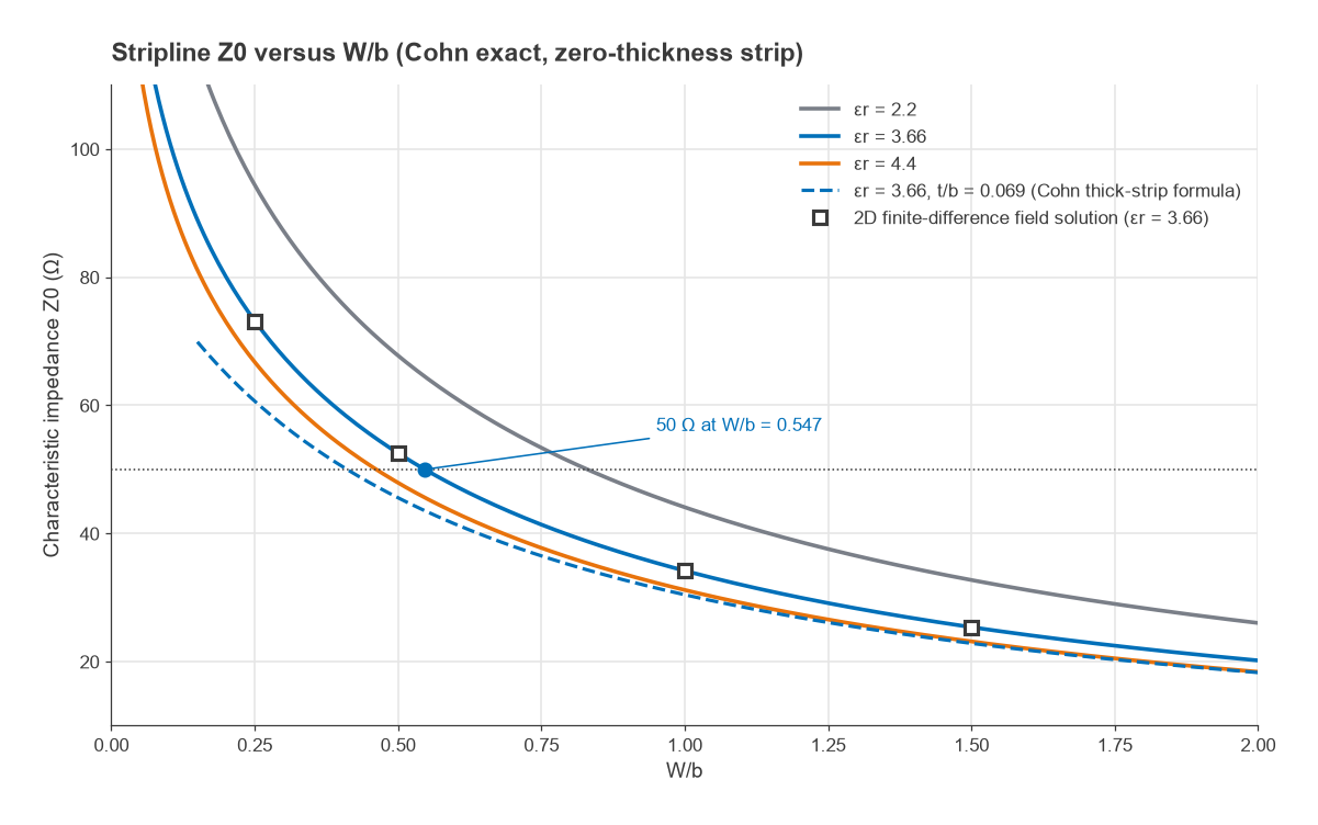
For a zero-thickness strip centred between infinite planes, conformal mapping gives an exact result in terms of the complete elliptic integral of the first kind K(k):
Z0 = (30π/√εr) · K(k)/K(k′), k = sech(πW/2b), k′ = tanh(πW/2b)
A widely used curve fit to this result avoids the elliptic integrals:
Z0 = (30π/√εr) · b/(We + 0.441b), with We/b = W/b − (0.35 − W/b)2 for W/b < 0.35 and We = W otherwise
For design the inverse is more useful. With x = 30π/(√εr Z0) − 0.441, the width is W/b = x when √εr Z0 < 120, and W/b = 0.85 − √(0.6 − x) otherwise.
Including strip thickness
Real copper has thickness, and it lowers the impedance noticeably when b is small. Cohn’s thick-strip formula, valid for W/(b − t) ≥ 0.35, is:
Z0 = (94.15/√εr) / [ (W/b)/(1 − t/b) + Cf′/(0.0885εr) ]
Cf′/(0.0885εr) = (1/π) [ 2q ln(q + 1) − (q − 1) ln(q2 − 1) ], with q = 1/(1 − t/b)
The first term in the bracket is the parallel-plate capacitance under the strip and the second is the fringing capacitance at its edges. For narrow strips, W/(b − t) < 0.35, the approximation commonly quoted from IPC-2141 is often used instead:
Z0 ≈ (60/√εr) ln[ 4b / (0.67π(0.8W + t)) ]
Its accuracy is limited, typically a few percent, so treat it as a starting point and confirm with a 2D field solver for production stack-ups.
Asymmetric (Offset) Stripline
When the strip is at height h1 above one plane and h2 below the other, a simple and reasonably accurate estimate treats the line as two symmetric striplines in parallel, one with plane spacing 2h1 and one with 2h2:
Z0,offset ≈ 2 Z0(2h1) Z0(2h2) / [ Z0(2h1) + Z0(2h2) ]
Each Z0(2h) uses the symmetric formula for a strip of the same width; physically, the capacitances of the two halves add. The nearer plane dominates, so for a fixed width the impedance drops as the strip moves off centre. The approximation ignores interaction between the halves at the strip edges and is typically within a few percent for moderate offsets.
As an example, take h1 = 0.2 mm, h2 = 0.4 mm, a thin strip and εr = 3.66. The parallel approximation gives 50 Ω at W = 0.293 mm. A 2D finite-difference field solution of the same geometry gives about 49.3 Ω, about 1.4 percent lower.
Losses in Stripline
All of the electric field is in the dielectric, so the dielectric attenuation is the full material value:
αd = π f √εr tanδ / c (Np/m)
Conductor loss depends on the surface resistance Rs = √(πfμ0/σ), which rises as √f because of the skin effect. For √εr Z0 < 120 a standard approximation is:
αc = [2.7×10⁻³ Rs εr Z0 / (30π(b − t))] · A (Np/m), A = 1 + 2W/(b − t) + (1/π)((b + t)/(b − t)) ln((2b − t)/t)
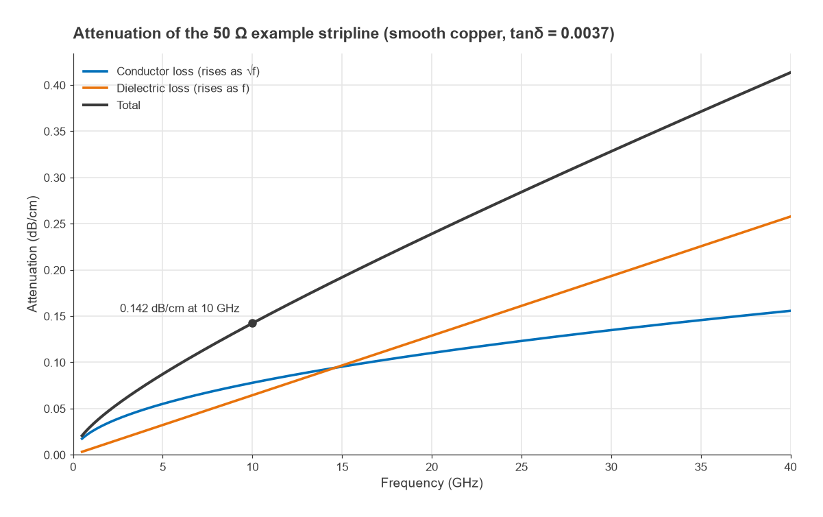
Multiply nepers by 8.686 to get decibels. For a given impedance and stack-up, a stripline is narrower than a microstrip because the strip sees ground on both sides, and current crowds onto both faces and the edges. Conductor loss per unit length is therefore usually higher than for an equivalent microstrip on the same total height, a point developed in transmission line losses. Copper roughness adds to the smooth-copper figure, often substantially at millimetre-wave frequencies.
Higher-Order Modes and Via Fences
Stripline supports higher-order waveguide-type modes once the plane spacing becomes a significant fraction of a wavelength. A common estimate of the lowest TE-type cutoff, with b and W in centimetres, is:
fc = 15 / (b√εr) · 1/(W/b + π/4) GHz
For thin boards this is far above the operating band. The more practical concern is the parallel-plate mode, which has no cutoff and is excited at every via transition and asymmetry. Ground vias along both sides of the line short the planes together and suppress it. Common guidance places them at a pitch of λ/10 to λ/20 of the wavelength in the dielectric at the highest frequency of interest, with the rows a few line widths from the strip so they do not change the impedance noticeably. Layout practice is covered in RF grounding and via stitching.
How to Design a Stripline Step by Step
- Choose the layers and find b, h1, h2, t and εr from the fabricator’s stack-up, using the permittivity value specified for design at your frequency.
- Estimate the width from the inverse thin-strip formula, then correct for thickness with Cohn’s formula or the narrow-strip approximation, whichever is in range.
- For an offset strip, use the parallel-combination estimate.
- Check the result with a 2D field solver, including any resin-rich layer next to the copper if the fabricator specifies one.
- Calculate delay and electrical length from vp = c/√εr, and losses from αc and αd.
- Place via fences on both sides and model the layer transitions, since these are where the line’s performance is usually lost.
Worked Example: 50 Ω Stripline at 10 GHz
Design a symmetric 50 Ω stripline with plane spacing b = 0.508 mm, 35 µm copper (t = 0.035 mm), εr = 3.66 and a typical loss tangent of 0.0037, then find its delay and loss at 10 GHz. Every figure below was checked numerically.
- Thin-strip width. √εr Z0 = 1.913 × 50 = 95.7, which is below 120, so W/b = x = 94.25/95.7 − 0.441 = 0.544. The exact elliptic-integral formula gives W/b = 0.547, so W = 0.278 mm for a zero-thickness strip.
- Thickness correction. t/b = 0.069. Solving Cohn’s thick-strip formula for 50 Ω gives W = 0.209 mm, with W/(b − t) = 0.44, inside its range. The 35 µm of copper has narrowed the 50 Ω trace by about a quarter. The narrow-strip approximation gives 0.201 mm, about 4 percent narrower.
- Field-solver check. A 2D finite-difference solution of the 0.209 mm geometry, extrapolated to zero cell size, gives about 50.2 Ω, which agrees with Cohn’s formula to within half a percent.
- Delay. vp = 3×10⁸/1.913 = 1.567×10⁸ m/s, so the delay is 6.38 ps/mm and the guided wavelength at 10 GHz is 15.67 mm.
- Loss at 10 GHz. Rs = 0.0261 Ω for copper, A = 3.07, giving αc ≈ 0.078 dB/cm. The dielectric term is αd ≈ 0.064 dB/cm. The total is about 0.142 dB/cm for smooth copper, so a 25 mm line loses roughly 0.36 dB.
- Higher-order modes and vias. The TE-type cutoff estimate is about 129 GHz, far above the band. A via pitch of λ/10 at 10 GHz is 1.57 mm; at 28 GHz it would be 0.56 mm.
For comparison, a 50 Ω microstrip on a single 0.254 mm layer of the same material is about 0.56 mm wide with a low-frequency εeff of 2.85. The stripline trace is less than half as wide, which helps routing density, but its narrower copper is the reason its conductor loss is relatively high. Microstrip widths can be checked with the microstrip calculator.
Stripline vs Microstrip vs Coplanar
| Property | Stripline | Microstrip | Grounded CPW |
|---|---|---|---|
| Mode | Pure TEM | Quasi-TEM | Quasi-TEM |
| Dispersion | None from geometry | Rises with frequency | Low |
| Radiation from line | None | Some, more at higher frequency | Low |
| Component access | Needs vias | Direct | Direct |
| Width for 50 Ω | Narrow | Wider | Set by gap |
| Tuning after build | Not possible | Possible | Possible |
Surface routes that connect components use microstrip or coplanar waveguide; buried routes that cross a dense board or must stay isolated use stripline. Stack-up material choices are covered in FR-4 vs Rogers laminates, and the circuit-level parameters of any line are explained in transmission line parameters.
Frequently Asked Questions
When should you use stripline?
Use it for inner-layer RF routing where isolation from other circuits, freedom from radiation and stable phase over a wide band are important. It also suits broadside and edge-coupled couplers, buried filters and matched-length lines. Avoid it where components must sit on the line or where post-build tuning is likely.
Why is stripline narrower than microstrip for the same impedance?
The strip has ground above and below, so its capacitance per unit length is roughly doubled compared with a strip that sees ground on one side only. It also sits fully in the dielectric. Both effects lower the impedance, so the strip must be narrower to reach 50 Ω.
Is stripline dispersive?
Not from its geometry. With one homogeneous dielectric the mode is pure TEM and εeff equals εr at all frequencies. Any remaining variation comes from the material’s own frequency dependence and from conductor loss.
What is offset stripline?
It is stripline with the conductor closer to one ground plane than the other. Its impedance can be estimated as the parallel combination of two symmetric lines with plane spacings 2h1 and 2h2, then confirmed with a field solver.
Related Topics
The transmission line theory hub links every line type, including waveguides for higher power and frequency. RF PCB layout shows how striplines fit into a full board, and EM simulation basics explains how to verify the transitions that a 2D formula cannot capture.