

Filter insertion loss is the reduction in signal power caused by placing a filter in a matched system, measured in the passband and expressed in dB as IL = −20log10|S21|. It is the first of a set of RF filter specifications, alongside passband ripple, return loss, rejection, shape factor, group delay and power handling, that together say how well a filter passes the wanted band and removes everything else.
A filter datasheet or a system requirement document lists these specifications because each one affects a different part of the radio. Insertion loss adds directly to receiver noise figure or subtracts from transmitter output power. Rejection decides how much interference reaches the next stage. Group delay matters for wideband modulated signals. This page defines each specification, shows how they are read from a measured or simulated response, and works through a single bandpass design so the numbers can be compared. It belongs to the RF filters section of the RF design reference.
The example filter
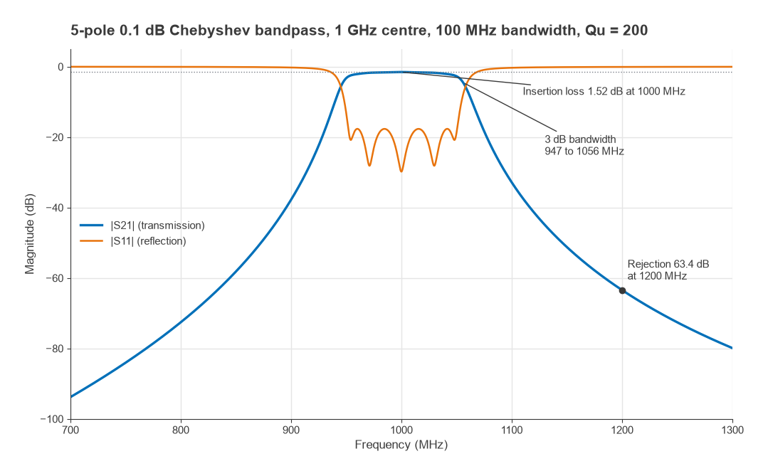
All the numbers on this page come from one circuit: a five-pole Chebyshev bandpass filter with 0.1 dB ripple, centred at f0 = 1000 MHz with a 100 MHz ripple bandwidth (fractional bandwidth FBW = 10%), in a 50 Ω system. The lowpass prototype values are g1 to g5 = 1.1468, 1.3712, 1.9750, 1.3712, 1.1468. Each resonator is given an unloaded Q of 200, a figure that is plausible for good lumped components or compact distributed resonators at 1 GHz. The response was computed by cascading the ABCD matrices of the five resonators. The design method itself is covered in LC filter design.
Insertion loss
Insertion loss compares the power delivered to the load with the filter in place against the power delivered without it:
IL = 10log10(Pwithout / Pwith) = −20log10|S21| dB (source and load matched to Z0)
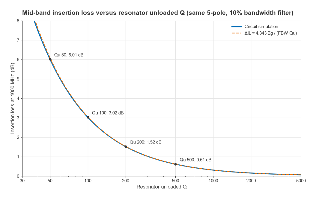
Two mechanisms contribute. Reflection sends some power back toward the source, set by the passband return loss. Dissipation turns some power into heat in the resonators, set by their unloaded Q. In a well-matched filter dissipation dominates. A standard approximation for the mid-band loss of a filter built from resonators with unloaded Qu is
ΔIL ≈ 4.343 × Σgk / (FBW × Qu) dB
For the example, Σg = 7.011, so ΔIL ≈ 4.343 × 7.011 / (0.10 × 200) = 1.52 dB. The circuit simulation gives 1.517 dB at 1000 MHz. The formula carries three lessons. Loss rises with the number of poles, so more selectivity costs more loss. Loss rises as bandwidth shrinks, so a 1% filter with the same resonators would lose about 15 dB. And loss falls only in proportion to Qu, which is why narrowband filters move to cavity, ceramic or acoustic resonators. The Q factor page explains where Qu comes from.
Why insertion loss matters in a receiver
A passive, matched filter at room temperature has a noise figure equal to its insertion loss. A 1.5 dB preselector in front of an LNA adds 1.5 dB to the system noise figure almost directly, as the cascaded noise figure calculation shows. In a transmitter, the same 1.5 dB after the power amplifier wastes about 29% of the output power. Both cases push designers to put low-loss filters at the antenna and to move sharper, lossier filtering to later stages.
Passband ripple, flatness and return loss
Ripple is the peak-to-peak variation of |S21| across the passband. A Chebyshev design sets it deliberately. A lossless 0.1 dB ripple filter has a passband return loss of at least
RL = −10log10(1 − 10−ripple/10) = −10log10(1 − 0.97724) = 16.4 dB
and the simulated filter shows 16.4 dB worst case across 951 to 1051 MHz, rising to about 30 dB at the reflection zeros. Loss changes the picture. With Qu = 200 the loss is no longer flat: it is 1.52 dB at the centre but 2.92 dB at the edges of the ripple band, because the resonators store more energy, and so dissipate more, where group delay is highest. Specifications therefore usually give a maximum insertion loss over the whole passband, not just at centre, and sometimes a separate “passband flatness” or “amplitude variation” limit. Return loss is often stated as VSWR; the conversion is on the VSWR and return loss page.
Bandwidth, rejection and shape factor
Bandwidth has several definitions and a specification should say which is meant. The ripple bandwidth is the range over which the response stays within the design ripple. The 3 dB bandwidth is measured 3 dB below the minimum insertion loss. For the example, the ripple band runs from 951.2 to 1051.2 MHz and the 3 dB band from 947.0 to 1056.0 MHz, a 3 dB bandwidth of 109.1 MHz. Bandpass responses built this way are geometrically symmetric about f0, so the band edges are not equally spaced from 1000 MHz in hertz.
Rejection, or stopband attenuation, is the attenuation at a named frequency or over a named range, relative to the input. The example filter gives 37.8 dB at 900 MHz, 32.8 dB at 1100 MHz and 63.4 dB at 1200 MHz. The asymmetry between 900 and 1100 MHz comes from the same geometric symmetry: 1100 MHz is closer to f0 on a logarithmic scale than 900 MHz is. A good rejection specification lists the frequencies of real interferers: the image, the local oscillator, the transmit band of a duplex system, or the harmonics of a power amplifier.
Shape factor summarises selectivity in one number, the ratio of a wide-attenuation bandwidth to the passband width. Using 60 dB and 3 dB points, the example measures 351.5 MHz / 109.1 MHz = 3.22. Using 40 dB and 3 dB it is 2.09. Lower is sharper, and 1.0 would be an ideal brick-wall filter. More poles, an elliptic response with transmission zeros, or higher Q all reduce shape factor. Acoustic filters reach very low shape factors in small packages, as described in SAW vs BAW filters.
Spurious passbands
Lumped filters keep rejecting far from the passband until parasitic elements take over. Distributed filters built from transmission-line resonators do not: a half-wave resonator is also resonant near 2f0, so a coupled-line filter can show a second passband there. The datasheet curve should extend far enough to show any such re-entry, especially when the filter is meant to remove harmonics. Microstrip filter design covers the usual remedies.
Group delay
Group delay is the time taken for the envelope of a narrowband signal to pass through the filter. It is the negative slope of the transmission phase with respect to angular frequency:
τg(ω) = −dφ21/dω
A constant group delay simply delays the signal. A delay that changes across the band delays some frequency components more than others, which distorts wideband modulation and shows up as error vector magnitude in a digital link. For the example filter the computed delay is 11.1 ns at 1000 MHz, rising to about 20 ns near the passband edges. A rough estimate at band centre is τ ≈ Σg / (2π × BW) = 7.011 / (2π × 100 MHz) ≈ 11.2 ns. Across the central 50 MHz the delay varies by 1.4 ns.
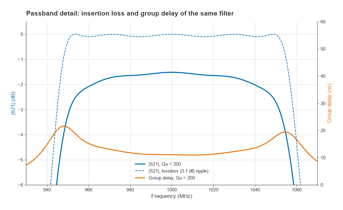
Two patterns are worth remembering. Sharper filters have larger delay and larger delay variation near the edges, so a signal that occupies the full passband sees the worst of it. And narrower filters have proportionally longer delay, which matters in feedback loops and in timing-sensitive systems. Specifications usually state group delay variation, in ns peak-to-peak over a stated bandwidth, rather than absolute delay.
Power handling and environmental specifications
Insertion loss is also a heat source. With 10 W at the input of the example filter, the output at 1000 MHz is 10 × 10−0.1517 = 7.05 W, about 0.01 W is reflected, and roughly 2.94 W is dissipated in the resonators. At the band edges, where loss is higher, the dissipation is higher still. Average power handling is set by how fast that heat leaves the structure. Peak power handling is set by voltage breakdown or, in acoustic filters, by stress in the piezoelectric material, and it can be the tighter limit for pulsed or high crest factor signals.
Other entries complete the specification: centre-frequency drift with temperature, usually given in ppm/°C; out-of-band return loss, which matters when the filter sits next to an amplifier that must stay stable at all frequencies; and, for filters in shared transmit and receive paths, passive intermodulation. In a duplexer the key additional figure is transmit-to-receive isolation.
Reading a filter specification
| Specification | Definition | Example value |
|---|---|---|
| Insertion loss (centre) | −20log|S21| at f0 | 1.52 dB |
| Insertion loss (passband max) | Worst case across the ripple band | 2.92 dB |
| Ripple (lossless design) | Peak-to-peak |S21| variation | 0.1 dB |
| Return loss | Minimum −20log|S11| in band | 16.4 dB |
| 3 dB bandwidth | Width at 3 dB below minimum IL | 109.1 MHz |
| Rejection | Attenuation at named frequencies | 37.8 dB at 900 MHz, 63.4 dB at 1200 MHz |
| Shape factor | BW60dB / BW3dB | 3.22 |
| Group delay | −dφ/dω at f0 | 11.1 ns |
| Group delay variation | Peak-to-peak over central 50 MHz | 1.4 ns |
Measured values come from a two-port vector network analyzer sweep. Insertion loss, return loss and group delay all derive from the same S-parameters, so a single calibrated measurement covers most of the table.
Frequently asked questions
What is insertion loss in a filter?
It is the drop in signal power, in dB, caused by inserting the filter between a matched source and load, measured at frequencies the filter is meant to pass. It combines power reflected at the input with power dissipated in the filter’s resonators, and it is equal to −20log|S21| when the system is matched.
What is group delay in a filter?
Group delay is the transit time of a signal’s envelope through the filter, found as the negative derivative of phase with respect to angular frequency. It peaks near the passband edges of sharp filters, and its variation across the band distorts wideband modulated signals.
Is insertion loss the same as attenuation?
Both are ratios of input to output power in dB, but the terms are used in different places. Insertion loss usually refers to the unwanted loss in the passband. Attenuation or rejection refers to the intended loss in the stopband.
How can a filter’s insertion loss be reduced?
Use resonators with higher unloaded Q, reduce the number of poles, or widen the bandwidth, since loss scales with Σg / (FBW × Qu). Good passband matching removes the smaller reflection component.
Related topics
The resonator quality behind insertion loss is explained in Q factor in RF circuits and parasitics of passive components. Filter implementations are compared in LC filter design, microstrip filter design and SAW vs BAW filters. Terms used here are defined in the wireless terms glossary.