

The Bode-Fano limit is a theoretical bound on broadband impedance matching. It states that for any load containing a reactive element, such as a resistor in parallel with a capacitor, no lossless matching network can keep the reflection coefficient low over an arbitrarily wide band: the integral of ln(1/|Γ|) over frequency cannot exceed a constant set by the load. Wider bandwidth always costs return loss, and the higher the load Q, the steeper the cost.
The limit tells a designer before any circuit is drawn whether a broadband specification is achievable at all. This page belongs to the impedance matching section of the RF design guide. It states the Bode-Fano integrals, works an example for a capacitive load, shows how close practical networks get, and then covers multi-section transformers and lossy matching, the two other tools for wide bandwidth.
Why Narrowband Matching Is Not Enough
A simple L-network gives a perfect match at one frequency, and its bandwidth is set by the network Q. The Pi and T networks add a degree of freedom that can raise or lower the Q, and a quarter-wave transformer matches resistive loads over a moderate band. All of them are point designs. When the requirement covers an octave or more, as in instrumentation amplifiers, wideband receivers, antennas and electronic warfare systems, the question changes from “how do I match?” to “how well can this load be matched over this band?” Bode and Fano answered that question.
The Bode-Fano Integral
Bode derived the result for a resistor shunted by a capacitor, and Fano generalized it to arbitrary loads. For a lossless, passive matching network between a resistive source and the load, the input reflection coefficient Γ(ω) must satisfy one of the following, depending on the load:
| Load | Bode-Fano constraint |
|---|---|
| R in parallel with C | ∫0∞ ln(1/|Γ(ω)|) dω ≤ π / (RC) |
| R in series with L | ∫0∞ ln(1/|Γ(ω)|) dω ≤ πR / L |
| R in series with C | ∫0∞ ω−2 ln(1/|Γ(ω)|) dω ≤ πRC |
| R in parallel with L | ∫0∞ ω−2 ln(1/|Γ(ω)|) dω ≤ πL / R |
The area under the curve of ln(1/|Γ|), which is return loss in nepers, is fixed. A designer can only choose where to spend it. Any part of the area spent outside the band of interest is wasted, so the best possible result puts |Γ| = 1 outside the band and a constant value Γmin inside it. For the parallel RC case over a band Δω this ideal gives
Δω · ln(1/Γmin) ≤ π / (RC), so Γmin ≥ exp[−π / (Δω RC)]
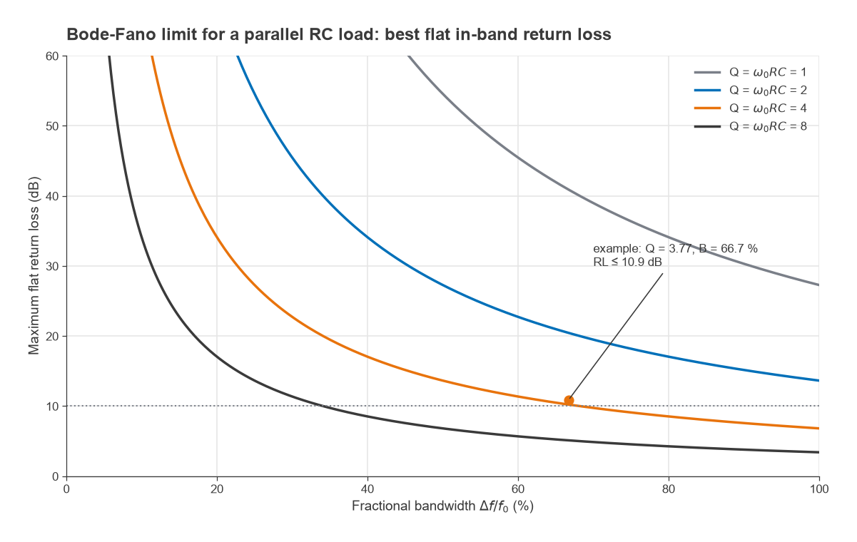
Writing the load Q at the band centre as Q = ω0RC and the fractional bandwidth as B = Δω/ω0 gives the compact form Γmin ≥ exp[−π / (Q·B)]. The product Q·B is all that matters. Doubling the bandwidth or doubling the load Q halves the exponent. Because the best return loss in decibels is RLmax = 8.686 π / (Q·B), it is halved as well.
Worked example: a capacitive load over 2 to 4 GHz
Model an amplifier input or a small antenna feed as R = 50 Ω in parallel with C = 4 pF, to be matched to 50 Ω from 2 to 4 GHz.
- Δω = 2π × 2 × 109 = 1.257 × 10¹⁰ rad/s and RC = 50 × 4 × 10−12 = 200 ps.
- π / (Δω RC) = π / 2.513 = 1.250.
- Γmin = exp(−1.250) = 0.287, so the best flat return loss is 10.9 dB, a VSWR of 1.80.
- Check with the Q form: Q = 2π × 3 × 109 × 200 × 10−12 = 3.77 at 3 GHz, B = 2/3, and Q·B = 2.51, the same exponent.
If the specification asks for 15 dB return loss across 2 to 4 GHz with this load, no lossless network can meet it. The options are to reduce C (a smaller device or a different feed), narrow the band, or accept loss. Halving the capacitance to 2 pF changes the exponent to 2.50 and the bound to 21.7 dB, which shows how strongly the result depends on the load.
How Close Real Networks Get
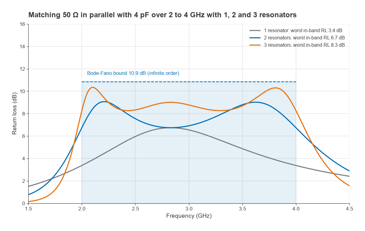
The Bode-Fano bound assumes a network of unlimited complexity that produces a perfectly rectangular reflection response. A finite network approaches it gradually. For the 50 Ω in parallel with 4 pF example, a numerical minimax optimization of bandpass ladders (alternating shunt and series resonators, with an ideal impedance transformer at the source side) gives the following worst-case in-band return loss:
- 1 resonator (a 0.79 nH shunt inductor tuning out the 4 pF): 3.4 dB.
- 2 resonators: 6.7 dB.
- 3 resonators: 8.3 dB.
- Unlimited order (Bode-Fano bound): 10.9 dB.
The first few sections give most of the improvement, and each additional one returns less. In practice two or three resonators are a common compromise, because every element adds loss, tolerance sensitivity and size. The ideal transformer in the model is usually realized with a tapped inductor, coupled lines, a transmission-line transformer or a Norton transformation of the ladder elements. Network synthesis methods such as real-frequency techniques produce these designs directly, but the optimizer result above is enough to show the trend.
Multi-Section Transformers for Resistive Loads
A purely resistive load has no reactance to constrain the integral, so in principle it can be matched over any bandwidth given a long enough network. The practical tool is a cascade of quarter-wave sections whose impedances step gradually from Z0 to ZL. Using the small-reflection approximation, the total reflection is Γ(θ) ≈ Σ Γn e−j2nθ, where θ is the electrical length of one section and Γn is the reflection at each step. Choosing the Γn fixes the shape of the response:
- Binomial (maximally flat): Γn proportional to the binomial coefficient C(N, n), giving ln(Zn+1/Zn) = 2−N C(N, n) ln(ZL/Z0). The response is as flat as possible at the centre frequency.
- Chebyshev (equal ripple): Γ(θ) = A e−jNθ TN(sec θm cos θ), where TN is the Chebyshev polynomial and sec θm = cosh[(1/N) cosh−1(|ln(ZL/Z0)| / 2Γm)]. The passband ripples between 0 and Γm, which buys much more bandwidth.
Worked example: 50 Ω to 12.5 Ω
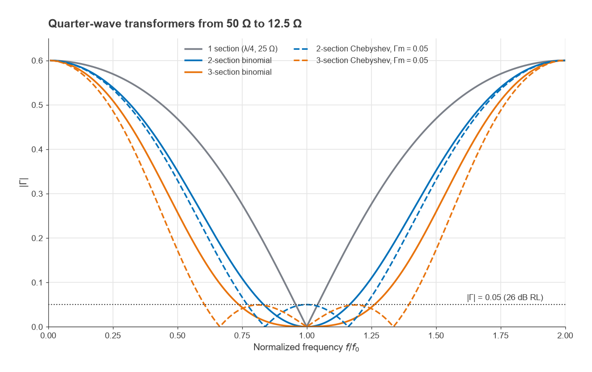
Match a 12.5 Ω load to 50 Ω with |Γ| ≤ 0.05 (26 dB return loss). The section impedances and the band where the exact cascade meets the specification are listed below.
| Design | Section impedances (Ω) | Bandwidth for |Γ| ≤ 0.05 |
|---|---|---|
| Single λ/4 | 25.00 | 8.2 % |
| 2-section binomial | 35.36, 17.68 | 33.1 % |
| 3-section binomial | 42.04, 25.00, 14.87 | 52.1 % |
| 2-section Chebyshev | 34.48, 18.13 | 46.1 % |
| 3-section Chebyshev | 39.48, 25.00, 15.83 | 79.0 % |
The Chebyshev three-section design covers roughly ten times the bandwidth of a single section for the same return loss. The cost is length: three quarter-wavelengths at the centre frequency instead of one, plus the line loss that comes with it. Tapered lines (exponential or Klopfenstein) are the continuous limit of the same idea and are common at microwave frequencies where length is cheap. The bandwidth formulas from the small-reflection theory are approximate; the values in the table come from cascading the exact line equations.
Lossy Matching and Other Trade-offs
The Bode-Fano limit applies only to lossless networks. Adding resistance breaks it, at the price of gain and noise. The simplest case is an attenuator in front of a poorly matched port: a pad of A dB improves the return loss by 2A dB, because the reflected wave passes through it twice. A port with 6 dB return loss behind a 3 dB pad shows 12 dB, but 3 dB of signal is lost and, at a receiver input, the noise figure rises by at least 3 dB. See RF attenuators for pad design.
- Resistive loading and feedback: shunt or feedback resistors flatten gain and match over decades of bandwidth in gain blocks, as described in broadband RF amplifier design.
- Balanced amplifiers: two identical stages between 90° hybrid couplers present a good match even when each stage is poorly matched, because reflections are steered into the coupler’s terminated port.
- Distributed amplifiers: absorbing the transistor capacitance into artificial transmission lines sidesteps the single-device limit by spreading the capacitance over many devices. See distributed amplifiers.
- Gain versus match: in amplifiers, a deliberate mismatch is often used to flatten gain across the band, trading return loss for flatness within the same Bode-Fano budget. The matching in filters and amplifiers page discusses this.
Frequently Asked Questions
What is the Bode-Fano limit?
It is a bound on how well a reactive load can be matched over a band with a lossless network. For a parallel RC load the integral of ln(1/|Γ|) over all frequencies cannot exceed π/(RC), so the best flat in-band reflection coefficient over a band Δω is exp[−π/(Δω RC)].
Does the Bode-Fano limit apply to resistive loads?
Not in the same way. A purely resistive load has no stored energy, so the bound becomes unlimited, and multi-section or tapered transformers can match it over very wide bands. Real resistive loads always have some parasitic reactance, which eventually sets a limit.
How many matching sections are worth using?
Usually two or three. In the example on this page, one, two and three resonators reach 3.4, 6.7 and 8.3 dB of a possible 10.9 dB. Further sections add loss and sensitivity for a shrinking improvement.
Can loss beat the Bode-Fano limit?
Yes, because the limit assumes a lossless network. Resistive pads, feedback and terminated couplers improve the match beyond the bound, but they reduce gain and, at the front of a receiver, raise the noise figure.
Related Topics
The impedance matching hub links every matching method on the site, including stub matching and the impedance matching calculator. For reading reflection data, see the Smith chart guide and VSWR and return loss. Broadband antenna feeds are discussed in antenna matching.