

A broadband RF amplifier is made wideband by setting its gain and impedance with frequency-independent elements, usually resistive negative feedback, rather than with resonant matching networks. Resistive shunt feedback, Darlington MMIC gain blocks, balanced amplifiers with quadrature hybrids and distributed amplifiers are the main techniques. Each trades some gain, noise figure or output power for flat gain and good match across one or more decades.
A narrowband amplifier can use reactive matching to extract the full maximum available gain of a transistor at one frequency. Across a decade that approach fails, because the available gain of a transistor falls with frequency and no lossless network can compensate it over a wide band without ripple. Broadband design accepts a lower, flat gain in exchange for bandwidth. This page explains the main techniques, works through design equations and a simulated example, and lists the steps from specification to layout. It sits in the RF amplifiers section of the RF design reference.
Why broadband design is different
The maximum available or stable gain of a transistor falls steadily with frequency, approaching 6 dB per octave as it nears fmax, while its input and output impedances are strongly reactive. A reactively matched amplifier designed for flat gain from 0.1 to 3 GHz would need a matching network that deliberately mismatches the device at low frequencies, where it has excess gain, by just the right amount at every frequency. The Bode-Fano limit, discussed under broadband matching, shows that the achievable match over a wide band is limited when the load contains a reactance. The practical answer is to reduce the gain to a level the device can deliver at the top of the band, and to use resistors to set both gain and impedance below that.
Typical broadband amplifier specifications include gain and gain flatness (for example ±0.5 dB or ±1 dB over the band), input and output return loss, noise figure, output P1dB and OIP3, and reverse isolation. Many of these are discussed on the RF amplifier datasheet page.
Resistive shunt feedback
The simplest broadband stage places a resistor Rf from the output (drain or collector) back to the input (gate or base). For an ideal transconductance device gm with infinite input and output impedance, the two-port with feedback in a Z0 system has
S11 = S22 = (1 − rg) / (1 + 2r + rg), S21 = −2(g − r) / (1 + 2r + rg)
where r = Z0/Rf and g = gmZ0. Both ports are matched simultaneously when
Rf = gmZ02, and then |S21| = gmZ0 − 1 = Rf/Z0 − 1
The gain is set by the ratio Rf/Z0, not by the device, and the match is set by the product of gm and Rf. A device with too much gm is degenerated with a series source or emitter resistor Re, which makes the effective transconductance roughly 1/Re. The matching condition then becomes
Z02 = Rf · Re
For a 15 dB target in 50 Ω, |S21| = 1015/20 = 5.62, so Rf = 50 × (1 + 5.62) = 331 Ω, the required gm is 6.62/50 = 132 mS, and the equivalent degeneration resistor is Re = 2500/331 = 7.55 Ω. These equations neglect the device’s output resistance and parasitic capacitances, so they give a starting point to refine in simulation.
Gain against bandwidth
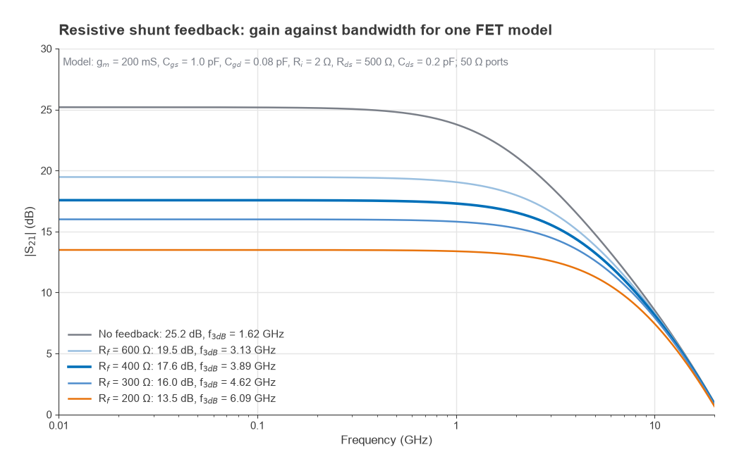
Feedback trades gain for bandwidth at nearly constant gain-bandwidth product. Figure 1 shows a FET equivalent circuit (gm = 200 mS, Cgs = 1.0 pF, Cgd = 0.08 pF, Ri = 2 Ω, Rds = 500 Ω, Cds = 0.2 pF) in a 50 Ω system with several feedback resistors:
| Rf | Low-frequency gain | 3 dB bandwidth | Input return loss (100 MHz) | Output return loss (100 MHz) |
|---|---|---|---|---|
| None | 25.2 dB | 1.62 GHz | 0 dB | 1.7 dB |
| 600 Ω | 19.5 dB | 3.13 GHz | 18.2 dB | 31.2 dB |
| 400 Ω | 17.6 dB | 3.89 GHz | 23.6 dB | 17.2 dB |
| 300 Ω | 16.0 dB | 4.62 GHz | 14.5 dB | 12.0 dB |
| 200 Ω | 13.5 dB | 6.09 GHz | 9.2 dB | 8.1 dB |
The linear voltage gain multiplied by the 3 dB bandwidth stays between 28.8 and 29.5 GHz for every case. The ideal formula predicts a match at Rf = 0.2 × 502 = 500 Ω. With the device’s finite 500 Ω output resistance included, the best input match moves to about 400 Ω, which gives 17.6 dB of gain, 23.6 dB input return loss at 100 MHz and gain within ±0.5 dB up to 1.38 GHz. That shift is typical of the gap between the hand equations and a full model.
Gain flatness
Even with feedback, the gain rolls off as Cgs and the Miller-multiplied Cgd load the input. With Rf = 400 Ω the model gives 17.57 dB at 100 MHz, 17.30 dB at 1 GHz, 16.56 dB at 2 GHz and 15.53 dB at 3 GHz, while input return loss degrades from 23.6 dB to 5.7 dB over the same range. Common ways to flatten the response are a small inductor in series with Rf, which reduces feedback at high frequencies and so raises the gain there; a series inductor at the drain for peaking; and a lossy input or interstage network whose loss falls with frequency. Each adds a frequency-dependent element and must be checked for stability over the full band, including far outside it.
Darlington MMIC gain blocks
The commercial broadband gain block is a resistive-feedback Darlington pair on one die. Two bipolar transistors (often SiGe HBT or GaAs HBT) are cascaded so that the first drives the base of the second, which multiplies their current gains and gives very high effective transconductance. An internal feedback resistor from output to input and emitter resistors set the gain and the 50 Ω match through the same relations, Z02 ≈ RfRe and |S21| ≈ Rf/Z0 − 1. Because the gain is fixed by resistor ratios on the die, it is repeatable from part to part and fairly insensitive to temperature.
Typical Darlington gain blocks are internally matched to 50 Ω and cover from tens of megahertz up to several gigahertz with gains of roughly 10 to 25 dB. They have a single combined output and bias pin, so they are biased through an RF choke and a resistor from the supply, as described in biasing RF transistors and MMICs. Their noise figure is usually several dB, higher than a dedicated LNA, because the feedback resistor adds thermal noise at the input. The comparison is developed further in LNA vs gain block vs PA.
Balanced amplifiers
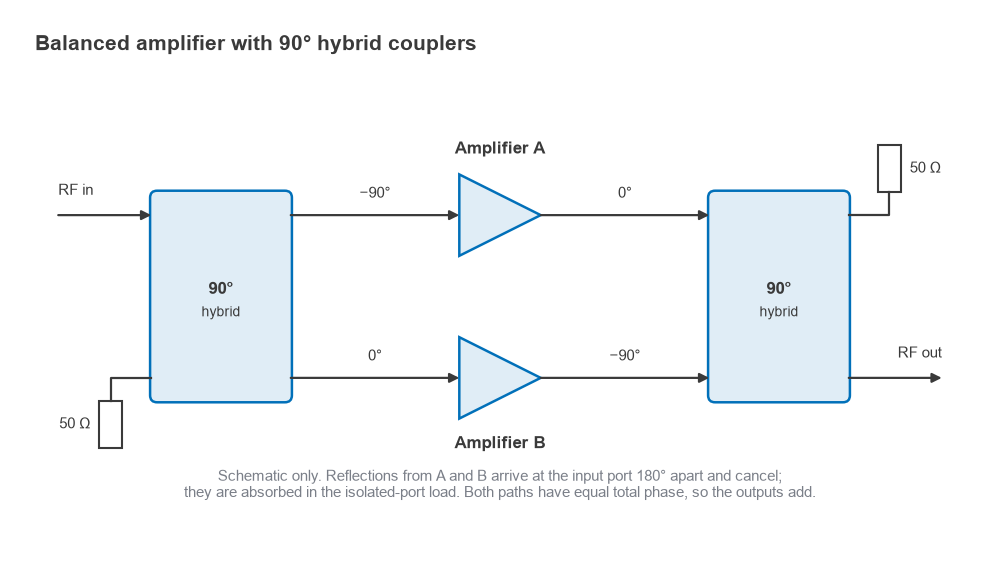
A balanced amplifier places two identical stages between a pair of 90° hybrid couplers. The input hybrid splits the signal into two paths 90° apart. The output hybrid recombines them with the opposite 90° shift, so the two paths have equal total phase and their outputs add. For ideal hybrids, the overall S-parameters in terms of the two stages A and B are
S11 = ½(S11A − S11B), S21 = −j½(S21A + S21B)
Reflections from the two stages travel back through the hybrid with a further 90° difference, arrive at the input port 180° apart and cancel. They add at the isolated port, where a 50 Ω termination absorbs them. If A and B are identical, the input and output match is perfect regardless of how badly each stage is matched. This frees each stage to be designed for noise figure, flat gain or output power instead of return loss.
Matching with imperfect stages
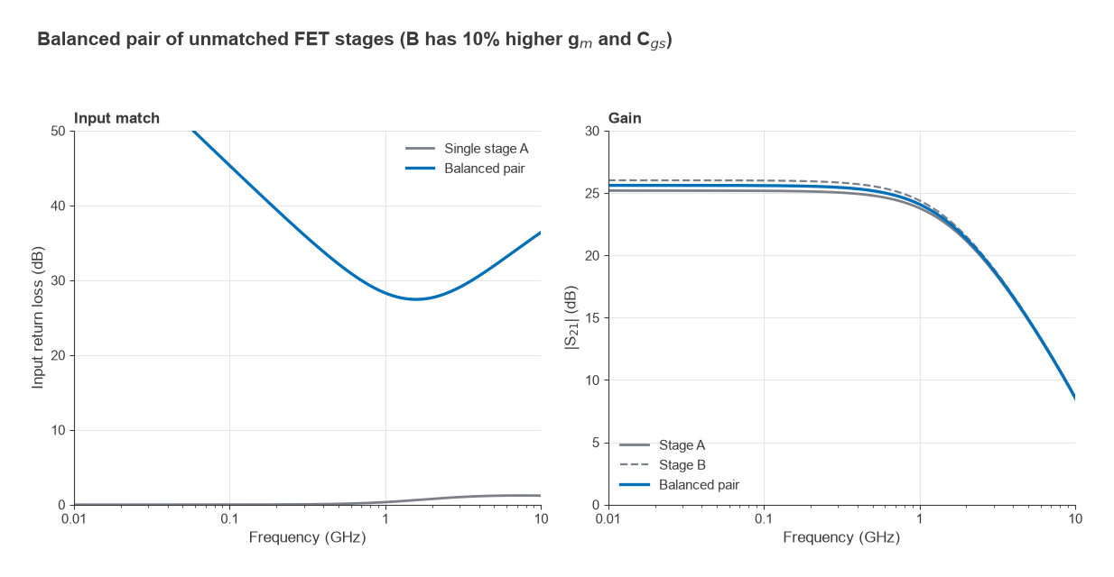
Figure 3 shows the effect with two open-loop FET stages from the earlier model, which have essentially no input match on their own (return loss below 1.3 dB everywhere). Stage B is given 10% more gm and Cgs to represent device spread. The balanced pair still has at least 27.4 dB of input return loss up to 3 GHz, and its gain sits between the two stages, 25.6 dB at 100 MHz. In practice, the bandwidth of the hybrids sets the limit. Lange and broadside-coupled hybrids typically cover about an octave or more; across a decade, the hybrid’s own amplitude and phase imbalance degrades the cancellation. Other benefits are 3 dB more output power and OIP3 than one stage, and graceful degradation if one stage fails. The costs are twice the DC power and the size and loss of the hybrids, covered under hybrid couplers.
Distributed amplifiers
For bandwidths of several decades up to tens of gigahertz, the distributed or travelling-wave amplifier absorbs the input and output capacitances of several transistors into artificial transmission lines, so that their gains add along the line while the capacitances become part of the line impedance. Gains are usually modest per unit, but bandwidth can extend close to the device cutoff frequency. The technique is covered on its own page, distributed amplifiers.
Design steps
- Fix the band, gain, flatness, return loss, noise figure and output P1dB or OIP3 targets.
- Check the device’s MAG or MSG at the top of the band. The flat gain target must sit comfortably below it, usually by several dB.
- Choose the topology: a single feedback stage or Darlington gain block for moderate gain; a balanced pair when match must be good and each stage is optimised for something else; cascaded stages when more gain is needed; a distributed design for multi-decade bandwidth.
- Calculate starting values: Rf = Z0(1 + |S21|) and Re = Z02/Rf for a feedback stage.
- Simulate with the full device model and adjust Rf, Re and any peaking inductors for flatness and match.
- Design the bias network so that its choke and blocking capacitors do not cause gain dips at the band edges.
- Check stability (K and μ) from well below to well above the band, then lay out with short ground paths as described in RF PCB layout, and measure on a VNA.
If the task is selecting a finished part rather than designing one, the companion guide how to choose a broadband RF amplifier covers the datasheet trade-offs.
Frequently asked questions
How do you make a wideband RF amplifier?
Use resistive negative feedback, or a ready-made Darlington gain block, to set the gain and the 50 Ω match with frequency-independent resistors, and keep the gain below what the transistor can deliver at the top of the band. For a better match or higher power, combine two stages in a balanced configuration. For multi-decade bandwidth, use a distributed amplifier.
What feedback resistor gives a 50 Ω match?
For an ideal transconductance stage, Rf = gmZ02, which gives |S21| = Rf/Z0 − 1. A 15 dB stage in 50 Ω needs about 331 Ω and an effective gm of about 132 mS. Device parasitics shift the optimum, so the value is refined in simulation.
Why is a balanced amplifier well matched?
The 90° hybrids make the reflections from the two stages arrive at the input 180° apart, so they cancel there and are dumped into the hybrid’s terminated port. With identical stages, the input return loss is limited only by the hybrid, not by the stages themselves.
Does feedback increase noise figure?
Yes, a resistive feedback network adds thermal noise at the input, so feedback amplifiers usually have a higher noise figure than reactively matched LNAs. A larger Rf adds less noise but gives more gain and less bandwidth. Where noise figure is critical, a reactively matched LNA or a balanced pair of low-noise stages is used.
Related topics
Broadband amplifier work connects to power gain definitions, stability, broadband matching and amplifier biasing. For noise and linearity in a chain of gain blocks, see cascaded noise figure and cascaded IP3. The section index is RF amplifiers, and terms are defined in the wireless terms glossary.