

A quarter-wave transformer is a section of transmission line one quarter wavelength long whose characteristic impedance is the geometric mean of the two impedances it connects, Z1 = √(Z0ZL). It works because a λ/4 line inverts impedance: a load ZL at one end appears as Z12/ZL at the other, which equals Z0 at the design frequency. It is the simplest distributed matching network, but it only matches real loads and its bandwidth shrinks as the impedance ratio grows.
The quarter-wave transformer is one of the main distributed techniques within impedance matching, alongside stub matching. It appears inside Wilkinson dividers, branch-line couplers, patch antenna feeds and power combiners. This page derives the design equation, walks through a microstrip example, and shows how multi-section binomial and Chebyshev transformers extend the bandwidth.
How a quarter-wave transformer works
The input impedance of a lossless line of characteristic impedance Z1 and electrical length θ, terminated in ZL, is
Zin = Z1 (ZL + jZ1 tan θ) / (Z1 + jZL tan θ)
When θ = 90°, tan θ goes to infinity and the expression reduces to Zin = Z12/ZL. Setting Zin equal to the source line impedance Z0 gives the design rule:
Z1 = √(Z0 ZL)
A physical picture helps. The wave reflected from the load end of the section and the wave reflected from the input step travel paths that differ by a half wavelength (a quarter wave out and a quarter wave back). With Z1 chosen as the geometric mean, the two reflections have equal magnitude and opposite phase, so they cancel. That cancellation is exact only at the frequency where the section is a quarter wavelength long, and at its odd multiples. The reflection coefficient page covers the single-step reflection used here.
Design steps
- Make sure the load is real at the point where the transformer will connect. If it is complex, add a length of line first (see below).
- Compute Z1 = √(Z0ZL).
- Find the line geometry for Z1 on the chosen medium, and its effective permittivity εeff.
- Compute the physical length ℓ = λg/4 = c/(4f0√εeff).
- Check the bandwidth against the requirement. If it is too narrow, use more sections.
- Simulate with step discontinuities and, for microstrip, the junction effects included, then trim the length.
Worked example: 50 Ω to 100 Ω at 2.4 GHz in microstrip
Match a 100 Ω resistive load to a 50 Ω line at 2.4 GHz on a substrate with εr = 3.5 and thickness h = 0.508 mm.
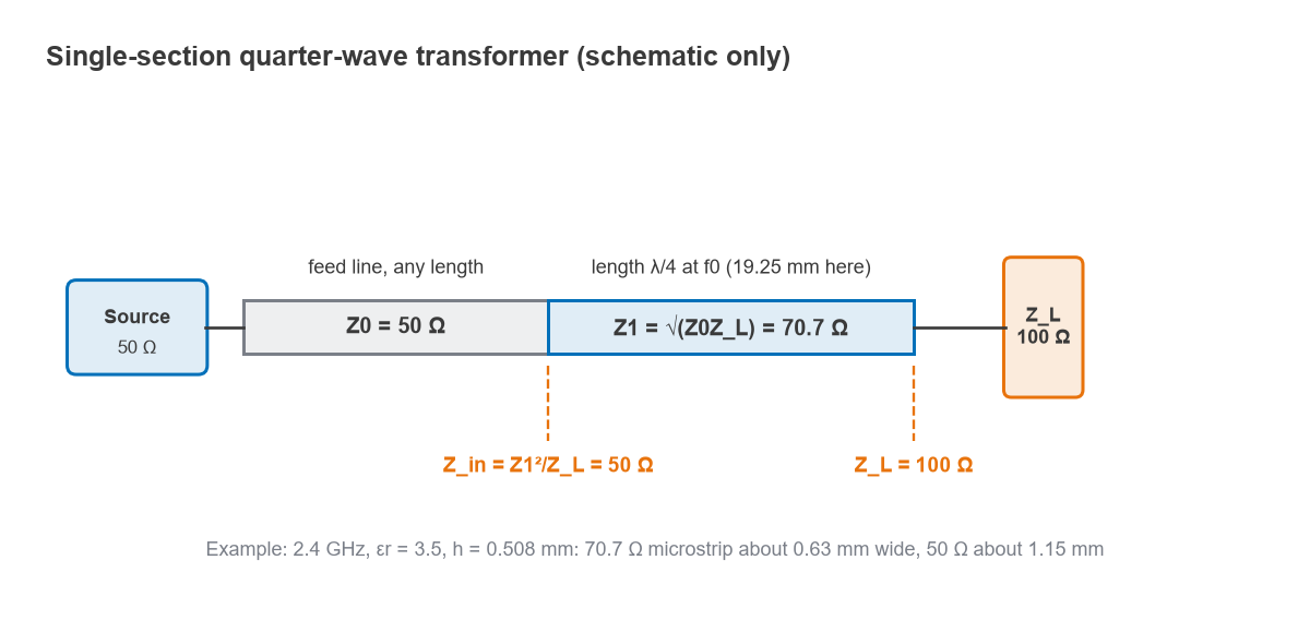
- Z1 = √(50 × 100) = 70.7 Ω.
- The Hammerstad and Wheeler synthesis equations (zero conductor thickness, no dispersion) give a width of about 0.63 mm for 70.7 Ω, with εeff ≈ 2.63. The 50 Ω feed is about 1.15 mm wide. The microstrip calculator uses the same equations.
- Guided wavelength λg = 299.79/(2.4 × √2.632) = 77.0 mm, so the section is 19.25 mm long.
- Check at the design frequency: Zin = 70.712/100 = 5000/100 = 50 Ω.
The width step from 1.15 mm to 0.63 mm adds a small shunt capacitance and some extra effective length at each end, so the final section is usually trimmed a little shorter in an EM simulation. The EM simulation page covers that step.
Matching a complex load
A quarter-wave transformer only matches a real impedance. For a complex load, move along the feed line until the impedance becomes real. On a line of impedance Z0 with standing-wave ratio S, the impedance is real and equal to Z0S at a voltage maximum and Z0/S at a voltage minimum.
For ZL = 100 + j50 Ω on a 50 Ω line, Γ = (ZL − Z0)/(ZL + Z0) = 0.447 at an angle of 26.6°, and S = (1 + 0.447)/(1 − 0.447) = 2.618. The first voltage maximum is at d = 26.6°/720° × λ = 0.0369λ from the load, where the impedance is 50 × 2.618 = 130.9 Ω. A transformer of √(50 × 130.9) = 80.9 Ω matches it. The alternative is to go on to the voltage minimum at 0.2869λ, where the impedance is 19.1 Ω, and use a 30.9 Ω transformer. The shorter total length usually gives the wider bandwidth. A Smith chart shows both points as the crossings of the constant-|Γ| circle with the real axis.
Bandwidth of a single section
Away from f0 the section is no longer a quarter wave and the cancellation is incomplete. The exact reflection magnitude at electrical length θ is
|Γ| = 1 / √{1 + [2√(Z0ZL) / |ZL − Z0| × sec θ]2}
Solving for the band where |Γ| stays below a maximum Γm, for TEM lines whose electrical length scales with frequency, gives the fractional bandwidth
Δf/f0 = 2 − (4/π) arccos[(Γm/√(1 − Γm2)) × 2√(Z0ZL) / |ZL − Z0|]
For the 50 to 100 Ω example with Γm = 0.1 (a 20 dB return loss): Γm/√(1 − Γm2) = 0.1005, the impedance factor is 2 × 70.71/50 = 2.828, their product is 0.2843, arccos(0.2843) = 1.2824 rad, and Δf/f0 = 2 − 1.6328 = 0.367. The match therefore holds 20 dB return loss over 36.7%, from about 1.96 to 2.84 GHz. Figure 2 shows how quickly that falls as the ratio grows: 17.1% for 50 to 200 Ω and 9.0% for 50 to 500 Ω, all at the same Γm. An exact line-equation sweep gives the same figures as the closed-form result.
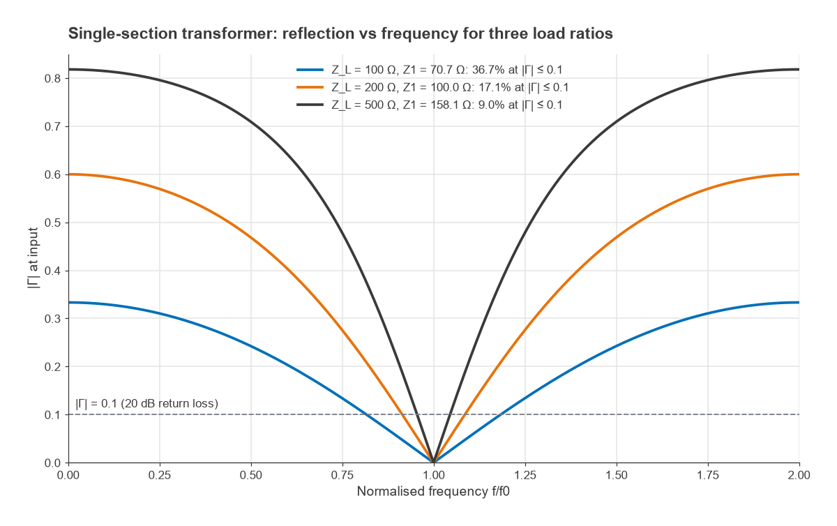
In a quasi-TEM medium such as microstrip, dispersion and the step discontinuities shift the response slightly, but the formula remains a good first estimate. The VSWR and return loss page converts between Γm, return loss and VSWR.
Multi-section transformers: binomial and Chebyshev
Splitting a large impedance step into several smaller steps, each a quarter wave long at f0, widens the bandwidth. Using the small-reflection approximation, the overall reflection is the sum of the reflections at each step, delayed by the line sections between them. The designer chooses the step sizes to shape that sum.
Binomial (maximally flat)
A binomial transformer sets the step reflections in proportion to the binomial coefficients, which makes the response as flat as possible at f0. For N sections:
ln(Zn+1/Zn) ≈ 2−N C(N, n) ln(ZL/Z0)
For 50 Ω to 200 Ω with N = 3, ln(200/50) = 1.386 and the coefficients are 1, 3, 3, 1 out of 8. That gives Z1 = 50 × 41/8 = 59.5 Ω, Z2 = 59.5 × 43/8 = 100.0 Ω and Z3 = 100.0 × 43/8 = 168.2 Ω. An exact simulation shows |Γ| ≤ 0.1 over 67.9% of f0, against 17.1% for a single 100 Ω section.
Chebyshev (equal ripple)
A Chebyshev transformer accepts a small, controlled ripple Γm in the passband in exchange for more bandwidth. The response follows a Chebyshev polynomial, |Γ(θ)| = Γm |TN(sec θm cos θ)|, where θm marks the band edge and is set by TN(sec θm) = |ln(ZL/Z0)|/(2Γm).
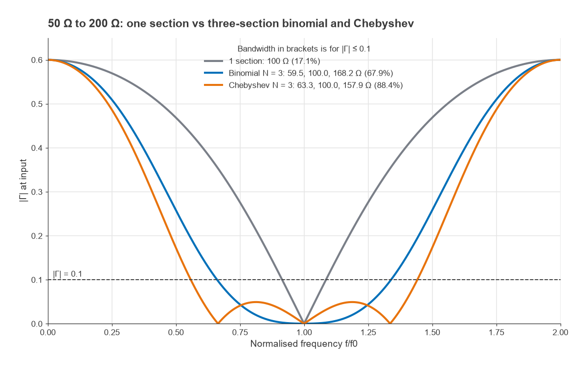
For the same 50 to 200 Ω match with N = 3 and Γm = 0.05: T3(sec θm) = 1.386/0.1 = 13.86, so sec θm = cosh[(1/3) arccosh 13.86] = 1.678 and θm = 53.4°. The ripple band runs from 53.4/90 = 0.594 f0 to 1.406 f0, about 81%. The section impedances come out at 63.3, 100.0 and 157.9 Ω. At the looser |Γ| ≤ 0.1 limit, the exact response covers 88.4%.
| Design (50 Ω to 200 Ω) | Section impedances | Bandwidth at |Γ| ≤ 0.1 | Total length at f0 |
|---|---|---|---|
| Single section | 100 Ω | 17.1% | λ/4 |
| Binomial, N = 3 | 59.5, 100.0, 168.2 Ω | 67.9% | 3λ/4 |
| Chebyshev, N = 3, Γm = 0.05 | 63.3, 100.0, 157.9 Ω | 88.4% | 3λ/4 |
The cost of more sections is length and loss: each section adds a quarter wave. Both multi-section designs are symmetric about the geometric mean of 100 Ω, a general property of these transformers. In practice the highest or lowest section impedance often limits the design, because very narrow or very wide lines are hard to build accurately. For tapered designs that extend this idea to a continuous line, and for the theoretical limit on bandwidth, see broadband matching.
Where quarter-wave transformers are used
- Power dividers and combiners. The 70.7 Ω arms of the Wilkinson divider are quarter-wave transformers from 50 Ω to 100 Ω.
- Antenna feeds. A patch antenna’s edge resistance is often a few hundred ohms; an inset feed or a quarter-wave section brings it to 50 Ω, as described in patch antenna design.
- Amplifier matching. At microwave frequencies a quarter-wave section combined with a short series line can replace a lumped L-network or pi network.
- Impedance inverters. In filters and Doherty amplifiers the same λ/4 property is used as an impedance inverter rather than a matching section.
Frequently asked questions
How does a quarter-wave transformer work?
A line one quarter wavelength long transforms a load ZL into Z12/ZL at its input. Choosing Z1 = √(Z0ZL) makes that equal to Z0, because the reflections from the two ends of the section cancel at the design frequency.
Can a quarter-wave transformer match a complex load?
Not directly. Add a length of line to reach a voltage maximum or minimum, where the impedance is real, or cancel the reactance with a stub, then use the transformer to match the remaining resistance.
How wide is the bandwidth of a quarter-wave transformer?
It depends on the impedance ratio. For a 2:1 ratio, 20 dB return loss holds over about 37% of the centre frequency; for 4:1 it is about 17%, and for 10:1 about 9%. Multi-section binomial or Chebyshev designs extend this considerably.
Related topics
Line fundamentals are covered in transmission line theory and transmission line terminations. For other distributed matching methods see single-stub and double-stub matching, and for the wider context see RF design and the wireless terms glossary.