


Impedance matching in RF filters and amplifiers means giving each block the source and load impedances it was designed around. A filter needs correct terminations to keep its passband shape, while an amplifier is matched at its input and output to trade gain, noise, stability and power. The two also interact, because a filter that reflects out of band presents a difficult load to the amplifier beside it.
The general idea is covered in what impedance matching is and why it matters. This page looks at what is different about the two most common blocks in a signal chain, with one filter example, one amplifier example and one example of the ripple the pair can produce.
Why Filters Need Correct Terminations
A passive LC filter has no gain and very little dissipation. It selects frequencies by reflecting unwanted power rather than absorbing it, and the element values are calculated for specific source and load resistances. The termination is therefore part of the design: change it and the response changes.
Example: A Butterworth Low-Pass Filter
Take a fifth-order Butterworth LC filter with a 900 MHz cutoff, designed for 50 Ω at both ends. Scaling the standard prototype values (0.618, 1.618, 2.000, 1.618, 0.618) gives shunt capacitors of 2.19 pF, 7.07 pF and 2.19 pF, and series inductors of 14.3 nH each.
Up to 750 MHz, the correctly terminated filter loses at most 0.65 dB. The table compares that case with two wrong loads, calculated by cascading ABCD matrices and using the transducer gain.
| Load (source remains 50 Ω) | Passband gain range, up to 750 MHz | Change at cutoff |
|---|---|---|
| 50 Ω (designed) | 0 dB to -0.65 dB | -3 dB point at 900 MHz |
| 100 Ω | -0.51 dB to -1.30 dB | Cutoff moves up |
| 20 Ω | -0.60 dB to -1.55 dB | Cutoff moves down |
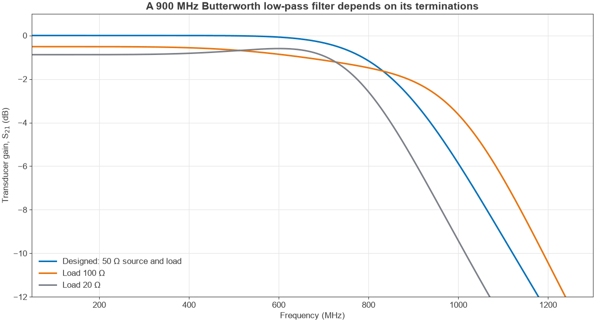
Resistive errors of this size are mild, but the filter’s flat passband has already gone. Reactive terminations do more harm, and high-order or narrow filters are more sensitive still. Narrow-band designs such as SAW and BAW filters are usually supplied with a recommended external matching network, because their terminals are often not close to 50 Ω. The RF filter specifications page explains how passband ripple and insertion loss are specified, always at stated terminations.
What a Filter Looks Like Outside Its Passband
In its stopband, a reflective filter has |S11| close to 1 with a phase that varies with frequency. Whatever connects to it sees an almost pure reactance. This matters in two ways: a mixer driven by that reflection can produce extra spurious products, and an amplifier can see a load near the edge of the Smith chart at a frequency where it still has gain. Designers handle this with an attenuator pad, an isolator or an absorptive filter such as a diplexer that terminates the unwanted band.
Matching an RF Amplifier
An amplifier’s ports are not naturally 50 Ω. A transistor generally has a low, capacitive input impedance and an output that depends on its bias and class. Matching networks transform the device impedance, and the choice of target depends on the amplifier’s job.
| Amplifier type | Input target | Output target |
|---|---|---|
| Low-noise amplifier | Near Γopt, for noise figure | Conjugate or near it, for gain and return loss |
| Gain block | Conjugate, wideband | Conjugate, wideband |
| Power amplifier | Conjugate, for drive and gain | Optimum load from load-pull |
Worked Example: Unilateral Gain Design
Consider a device with these illustrative S-parameters in a 50 Ω system, which are not taken from any real part:
S11 = 0.6∠-120°, S21 = 4.0∠70°, S12 = 0.05∠40°, S22 = 0.5∠-40°
Stability comes first. The Rollett factor is K = 1.30 with |Δ| = 0.36, and μ = 1.18, so the device is unconditionally stable and a simultaneous conjugate match exists. See amplifier stability for the definitions.
If S12 is ignored, the transducer gain splits into three separate parts:
- Device: G0 = |S21|2 = 16, or 12.04 dB
- Source match: GS,max = 1 / (1 – |S11|2) = 1.56, or 1.94 dB
- Load match: GL,max = 1 / (1 – |S22|2) = 1.33, or 1.25 dB
The total is 15.23 dB. Matching alone has added 3.19 dB to the 12.04 dB seen in a plain 50 Ω system. The networks must present ΓS = S11* and ΓL = S22*, which correspond to ZS = 16.3 + j26.5 Ω and ZL = 77.5 + j66.4 Ω.
How Accurate Is the Unilateral Assumption?
The unilateral figure of merit is U = |S12S21S11S22| / ((1 – |S11|2)(1 – |S22|2)) = 0.125. The true gain then lies between -1.02 dB and +1.16 dB of the unilateral estimate, a span of about 14.2 dB to 16.4 dB.
An exact simultaneous conjugate match resolves this. It needs ΓS = 0.703∠132.5° and ΓL = 0.626∠60.6°, and gives 15.75 dB, inside the predicted range. Power gain definitions explains how this relates to available and operating gain.
Gain Circles and the Noise Trade-Off
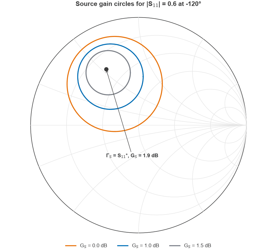
The maximum is a single point, but gain falls slowly around it. Figure 2 plots constant source gain circles for this device. The 0 dB circle passes through the centre of the chart, because a 50 Ω source gives no matching gain at all. The 1.5 dB circle shows that a designer can give up 0.44 dB and still have a wide choice of ΓS.
That freedom is what makes an LNA design possible. If Γopt falls inside a usable gain circle, the source can be set near it, accepting slightly less gain for lower noise. The input mismatch that results can be reduced with inductive source degeneration, which moves the conjugate match point toward Γopt with no noise penalty in the ideal case. How to choose an LNA covers the specifications involved.
When Filter and Amplifier Meet
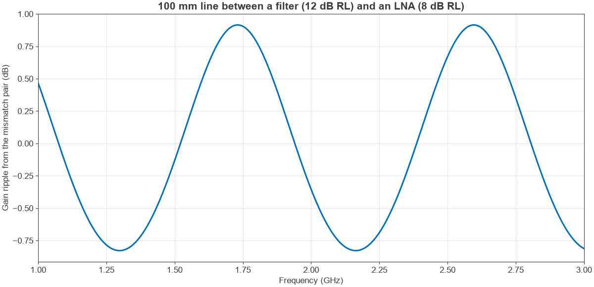
Blocks that each pass their own specification can still disappoint when connected. Two reflections with a line between them form a resonator, and the gain varies with the phase around that loop. The peak-to-peak ripple for a lossless line follows directly from the two reflection magnitudes:
Ripple = 20 log10((1 + |Γ1Γ2|) / (1 – |Γ1Γ2|))
Worked Example: Filter Into an LNA
Suppose a filter with 12 dB return loss drives an LNA with 8 dB return loss through 100 mm of line with εeff = 3.0. The reflection magnitudes are 0.251 and 0.398, and their product is 0.100.
The gain then swings between +0.92 dB and -0.83 dB, which is 1.74 dB peak to peak. The ripple period is v / 2L = 865 MHz, as Figure 3 shows. A longer line brings the ripple closer together, which can put several cycles across one wide channel, and the associated group delay variation affects wideband modulation.
Practical Techniques
Several measures control these interactions, and most combine well with the others:
- Keep lines short between poorly matched blocks, so the ripple period is wider than the band of interest.
- Put a small attenuator between sensitive stages where gain and noise allow it. A 3 dB pad improves return loss by 6 dB.
- Use balanced amplifiers with 90 degree hybrid couplers to get good port matching even when each device is deliberately mismatched.
- Use isolators at the output of a power amplifier when the load varies.
- Simulate the whole chain from measured S-parameters, including stopbands, instead of checking each block alone.
- Check stability out of band, since a filter’s stopband reflection can present passive terminations of any phase.
Frequently Asked Questions
Why does a filter’s response change with load impedance?
Its element values are derived for particular terminations, and it works by controlled reflection. Changing a termination changes those reflections, so the passband shape, the cutoff frequency and the group delay all move.
Should an LNA be power matched or noise matched?
Usually it is placed close to the noise match, since input losses and noise figure matter most in a receiver front end. Good LNA designs bring the two points close together, for example with source degeneration, so that both noise and return loss are acceptable.
Is a power amplifier output conjugate matched?
Not normally. Its output is matched to the load that gives the required power, efficiency and linearity, and this load is found by load-pull or from the load-line. The output return loss can be poor as a result.
Where should a filter sit relative to an amplifier?
It depends on the priority. A filter before an LNA protects the receiver from large signals but adds its loss directly to the noise figure. A filter after the LNA costs less noise but leaves the LNA exposed. Many receivers use a filter on each side.
Related Topics
This page sits under RF amplifiers and connects to RF filters. For matching circuits themselves, see L-network matching and broadband matching, or use the impedance matching calculator.