Distributed (Traveling-Wave) Amplifiers

A distributed amplifier, also called a traveling-wave amplifier, is a broadband amplifier in which several transistors are connected between two artificial transmission lines so that their input and output capacitances become part of the lines instead of limiting bandwidth. The input signal travels down the gate line and drives each transistor in turn, and the output currents add in phase on the drain line as they travel toward the load.

The result is gain that extends from near DC to a large fraction of the transistor cutoff frequency, at the cost of modest gain per device, more die area and lower efficiency than a tuned stage. Distributed amplifiers are the usual choice when an application needs a decade or more of bandwidth, such as instrumentation, optical modulator drivers and wideband receivers. This page explains how the artificial lines work, derives the gain and gain-bandwidth expressions, and works through a four-cell example checked by circuit simulation. It sits in the RF amplifiers section of the RF design guide.

How a Distributed Amplifier Works

In a conventional single-stage amplifier, the input capacitance of the transistor has to be charged through the source resistance, which sets a pole at roughly 1/(2πR_sC_gs). Adding more transistors in parallel raises the transconductance but raises the capacitance by the same factor, so the gain-bandwidth product stays near the transistor f_T. The distributed amplifier breaks this limit by never presenting the capacitances in parallel.

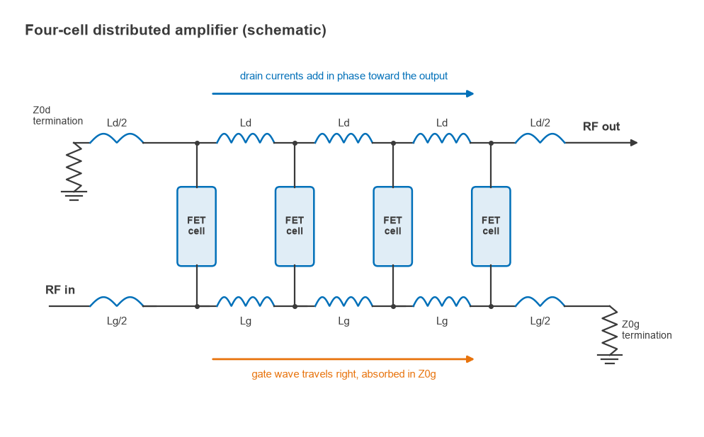
Four-cell distributed amplifier with gate and drain inductor ladders, FET cells and resistive terminations — Figure 1: Four-cell distributed amplifier (schematic only). Gate and drain inductors combine with device capacitances to form two artificial transmission lines.

Each transistor gate is connected to a node of a ladder of series inductors. The inductors and the gate-source capacitances together form a lumped approximation of a transmission line, the gate line, terminated at its far end in its characteristic impedance. The drains are connected in the same way to a second ladder, the drain line, which is terminated at its input end and delivers power to the load at its output end.

A signal applied to the gate line travels from cell to cell. Each transistor converts its gate voltage into a drain current, and that current launches two waves on the drain line, one toward the output and one toward the drain termination. If the phase delay per section on the drain line equals that on the gate line, every forward-travelling contribution arrives at the output in phase with the others and they add. The reverse waves do not line up and are absorbed in the drain termination. Whatever signal reaches the end of the gate line is absorbed in the gate termination.

Artificial Transmission Lines

A ladder of series inductors L and shunt capacitors C is a constant-k low-pass filter. Well below its cutoff it behaves like a uniform transmission line with

Z₀ = √(L/C) f_c = 1/(π√(LC))

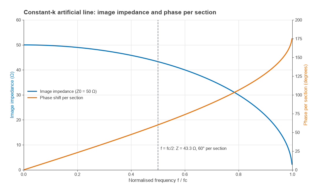
where f_c is the cutoff (Bragg) frequency of the ladder. Near cutoff the line is no longer smooth. The image impedance of a mid-shunt section falls as Z_I = Z₀√(1 − (f/f_c)²), and the phase shift per section rises as φ = 2 arcsin(f/f_c), reaching 180° at cutoff. A fixed resistive termination therefore matches the line well only up to perhaps half of f_c; designers use m-derived end sections to keep the termination closer to the image impedance over more of the band.

Image impedance and phase shift per section of a constant-k LC ladder versus normalised frequency — Figure 2: A 50 Ω constant-k ladder. At half the cutoff frequency the image impedance has fallen to 43.3 Ω and each section adds 60° of phase.

On the gate line C is the transistor C_gs. On the drain line C is the drain-source capacitance C_ds, which is normally much smaller, so an extra padding capacitor is added at each drain node to equalise the phase velocity of the two lines. With equal Z₀ on both lines the condition is simply C_ds + C_pad = C_gs. The same ideas underlie ordinary transmission line parameters, and the general theory is in transmission line theory.

Gain of a Distributed Amplifier

For an ideal lossless amplifier with N cells, transconductance g_m per cell and gate and drain line impedances Z_0g and Z_0d, each cell injects g_mV_in into the drain line, half of which travels toward the load. The output voltage is N g_mV_inZ_0d/2 and the available power gain is

G = g_m² N² Z_0g Z_0d / 4

Gain grows as N² in this limit, which is the main attraction. Real lines have loss. On the gate line the input resistance R_i in series with C_gs absorbs power, and on the drain line the output resistance R_ds loads every node. If A_g and A_d are the attenuations per section in nepers, the gain becomes

G = (g_m² Z_0g Z_0d / 4) × (e^−NA_g − e^−NA_d)² / (e^−A_g − e^−A_d)²

with the low-frequency approximations A_g ≈ ω²C_gs²R_iZ_0g/2 and A_d ≈ Z_0d/(2R_ds). This expression appears in standard microwave texts. It reduces to the lossless form when both attenuations go to zero and to g_m²Z₀²/4 for one cell.

Optimum number of cells

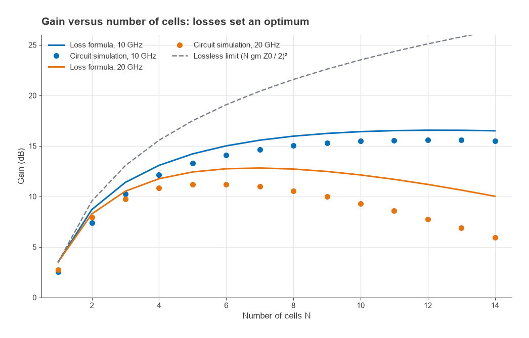
Adding cells adds current to the drain line, but every added section also attenuates the signal already travelling on both lines. Differentiating the lossy gain expression with respect to N gives the optimum

N_opt = ln(A_d/A_g) / (A_d − A_g)

Because A_g rises with the square of frequency, the optimum falls as the top of the band rises. Practical designs commonly use somewhere between three and ten cells; beyond the optimum, extra cells cost area and DC power and reduce gain at the upper band edge.

Gain versus number of cells at 10 and 20 GHz from the loss formula and circuit simulation, with the lossless limit — Figure 4: Gain versus cell count. Line losses cap the N² growth; at 20 GHz the gain stops rising at about six cells.

Gain-Bandwidth of the Distributed Amplifier

With Z₀ = √(L/C_gs), the gate line cutoff can be written f_c = 1/(πZ₀C_gs). The lossless voltage gain is A_v = N g_mZ₀/2. Their product is

A_v × f_c = N g_m / (2πC_gs) = N f_T

A lumped amplifier built from the same devices is limited to a voltage gain-bandwidth near f_T, however many devices are placed in parallel. The distributed amplifier scales it by the number of cells, which is why the topology can reach bandwidths close to the device cutoff while still providing useful gain. Losses reduce the benefit, and the choice of Z₀ trades gain against bandwidth: a higher impedance raises g_mZ₀ but lowers f_c for the same C_gs. Device choice matters for the same reason, and the RF transistor technologies page compares f_T and output resistance across GaAs, GaN, SiGe and CMOS.

Worked Example: a Four-Cell Design

Take a generic FET cell with g_m = 60 mS, C_gs = 0.2 pF, R_i = 8 Ω, R_ds = 150 Ω and C_ds = 0.05 pF, and design for 50 Ω lines.

Simulated S21 versus frequency of the example distributed amplifier for 2, 4, 6 and 8 cells — Figure 3: Simulated |S21| of the example design (gm 60 mS, Cgs 0.2 pF, 50 Ω lines). Four cells give 11.1 dB at low frequency and a 3 dB bandwidth near 25.8 GHz.

Line inductance: L = Z₀²C_gs = 2500 × 0.2 pF = 0.5 nH per section, used on both lines.
Drain padding: C_pad = 0.2 − 0.05 = 0.15 pF per drain node.
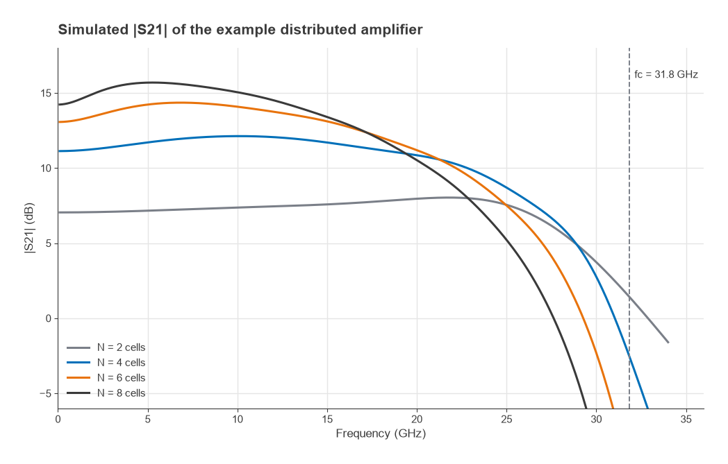
Line cutoff: f_c = 1/(π × 50 × 0.2 pF) = 31.8 GHz.
Device f_T = 0.06/(2π × 0.2 pF) = 47.7 GHz.
Lossless gain with N = 4: A_v = 4 × 0.06 × 50/2 = 6, or 15.6 dB, and the voltage gain-bandwidth N f_T = 191 GHz.

Now add the losses. The drain attenuation is A_d = 50/(2 × 150) = 0.167 Np, or 1.45 dB per section, independent of frequency in this simple model. The gate attenuation at 20 GHz is A_g = (2π × 20 GHz)² × (0.2 pF)² × 8 × 50/2 = 0.126 Np. The lossy formula then gives about 11.8 dB for four cells at 20 GHz, and N_opt = ln(0.167/0.126)/(0.167 − 0.126) ≈ 6.9 cells. At 10 GHz the gate loss is a quarter as large and the optimum moves out to about 12 cells.

A nodal circuit simulation of the same ladder, with half-inductor end sections, 50 Ω source, load and terminations, gives 11.1 dB at low frequency, a peak of 12.1 dB near 10 GHz, 10.9 dB at 20 GHz and a 3 dB bandwidth of about 25.8 GHz for four cells. At 20 GHz the simulated gain is flat at about 11.2 dB for five and six cells and falls for more, close to the formula’s prediction. The simple formula reads slightly high near cutoff because it ignores the falling image impedance and the mismatch to the fixed terminations, which is one reason designers confirm every distributed amplifier in a full circuit simulator before layout.

Practical Design Considerations

Cascode cells and gate capacitors

Replacing each common-source FET with a cascode pair raises the output resistance, which cuts drain line loss, and reduces feedback through the gate-drain capacitance. A small series capacitor in each gate connection divides down the effective C_gs seen by the gate line, which raises its cutoff at the cost of gain. Both techniques are widely used in monolithic designs.

Terminations, bias and low-frequency response

The drain termination usually doubles as the DC feed, through a large off-chip inductor or a bias tee, so its value and the decoupling around it set the low-frequency corner. The terminations also give good input and output return loss over much of the band, since both ports look into a resistively terminated line. Stability still has to be checked across the full frequency range, as described in amplifier stability and the K factor, and bias networks are covered in RF amplifier biasing.

Noise, power and efficiency

The gate termination contributes thermal noise that travels back toward the input of each cell, so the noise figure of a distributed amplifier is usually worse at the low end of the band and higher overall than a narrowband LNA built on the same process. Half of each drain current flows into the drain termination, which wastes power and limits efficiency. Output power is limited by the last cells, which see the largest voltage swing; tapering the drain line impedance along its length can spread the swing more evenly. For these reasons distributed amplifiers are chosen for bandwidth, not for noise or efficiency, a trade summarised in LNA vs gain block vs PA.

Where distributed amplifiers are used

Typical uses include wideband test equipment front ends, electronic warfare receivers, drivers for optical modulators in fibre links, and general gain stages covering several octaves. Most are built as MMICs, since the small inductors and well-controlled device parasitics are easier to realise on a monolithic process; see MMIC vs RFIC. Alternatives with less bandwidth but better noise or efficiency are covered in broadband RF amplifier design and broadband matching. At millimetre-wave frequencies the same principles reappear in the wideband stages described in mmWave radio architectures.

Frequently Asked Questions

How does a distributed amplifier work?

The input signal travels along an artificial transmission line formed by series inductors and the transistor input capacitances, driving each transistor in turn. The transistor output currents are collected on a second artificial line with matched phase velocity, so their forward waves add in phase at the output while reverse waves are absorbed in a termination.

Why is a distributed amplifier so broadband?

The transistor capacitances are absorbed into transmission lines rather than appearing in parallel at a single node, so they do not form a dominant RC pole. Bandwidth is then limited by the cutoff of the artificial lines and by line losses, and the voltage gain-bandwidth product scales roughly with the number of cells times f_T.

How many stages does a distributed amplifier need?

There is an optimum set by gate and drain line losses, N_opt = ln(A_d/A_g)/(A_d − A_g), evaluated at the top of the band. In the worked example it is six to seven cells at 20 GHz. Practical designs often use three to ten cells.

What are the drawbacks of distributed amplifiers?

Gain per device is low, half the output current is lost in the drain termination, efficiency is poor, and noise figure is higher than a tuned LNA. They also need more die area. They are used where bandwidth outweighs these costs.