

Stub matching is a distributed matching technique that cancels a load’s mismatch with a short-circuited or open-circuited length of transmission line connected in shunt (or series) with the main line. To design a single-stub match, move from the load along the line until the real part of the admittance equals Y0, then add a stub whose susceptance cancels the remaining imaginary part. Two numbers define the design: the stub position d and the stub length ℓ.
Stubs are the microwave counterpart of the lumped L-network and sit within the wider topic of impedance matching. Unlike the quarter-wave transformer, a stub match handles complex loads directly and needs only lines of one characteristic impedance. This page covers the Smith chart procedure, the closed-form equations, a worked microstrip example, double-stub tuners and radial stubs.
How a single shunt stub works
Shunt elements add admittances, so the design is easiest in admittance terms. Moving along a lossless line from the load toward the generator rotates the normalised admittance around a circle of constant |Γ| on the Smith chart. Somewhere on that circle, twice per half wavelength, the circle crosses the g = 1 circle, where the admittance is y = 1 + jb. A shunt stub with susceptance −jb placed at that point leaves y = 1, a match.
A stub is just a line terminated in a short or an open, so its input is purely reactive. For a stub of characteristic impedance Z0 and length ℓ, with β = 2π/λ:
- Open-circuited stub: ystub = j tan(βℓ)
- Short-circuited stub: ystub = −j cot(βℓ)
Any susceptance from −∞ to +∞ can be produced by choosing ℓ between 0 and λ/2, so a single stub can match any load with non-zero real part, given freedom to place it.
Smith chart procedure
- Normalise the load: zL = ZL/Z0, and plot it.
- Convert to admittance by reflecting the point through the chart centre to get yL. From here on, read the chart as an admittance chart.
- Draw the constant-|Γ| circle through yL.
- Rotate clockwise (toward the generator) until the circle meets the g = 1 circle. There are two crossings, 1 + jb and 1 − jb. Read the distance travelled on the wavelengths-toward-generator scale: that is the stub position d.
- The stub must supply −jb. For a shorted stub, start at the short-circuit admittance point (y = ∞, the right-hand end of the real axis) and rotate clockwise until you reach −jb on the outer circle. For an open stub, start at y = 0 (the left-hand end). The rotation gives ℓ.
- Check: at the stub junction, y = (1 + jb) + (−jb) = 1.
Closed-form design equations
For a load ZL = RL + jXL on a line Z0, let t = tan(βd). Requiring the real part of the admittance at d to equal Y0 gives, for RL ≠ Z0:
t = [XL ± √(RL((Z0 − RL)2 + XL2)/Z0)] / (RL − Z0)
with d/λ = (1/2π) arctan t for t ≥ 0 and d/λ = (1/2π)(π + arctan t) for t < 0. The susceptance at that point is
B = [RL2t − (Z0 − XLt)(XL + Z0t)] / {Z0[RL2 + (XL + Z0t)2]}
and the stub must provide −B. The lengths follow from the stub admittances above: ℓopen/λ = −(1/2π) arctan(B/Y0) and ℓshort/λ = (1/2π) arctan(Y0/B), adding λ/2 to any negative result.
Worked example: 25 − j40 Ω at 2.4 GHz
Match a load of 25 − j40 Ω, such as a small capacitive antenna, to a 50 Ω microstrip line at 2.4 GHz. The normalised load is zL = 0.5 − j0.8, so yL = 1/zL = 0.562 + j0.899, and |Γ| = 0.555.
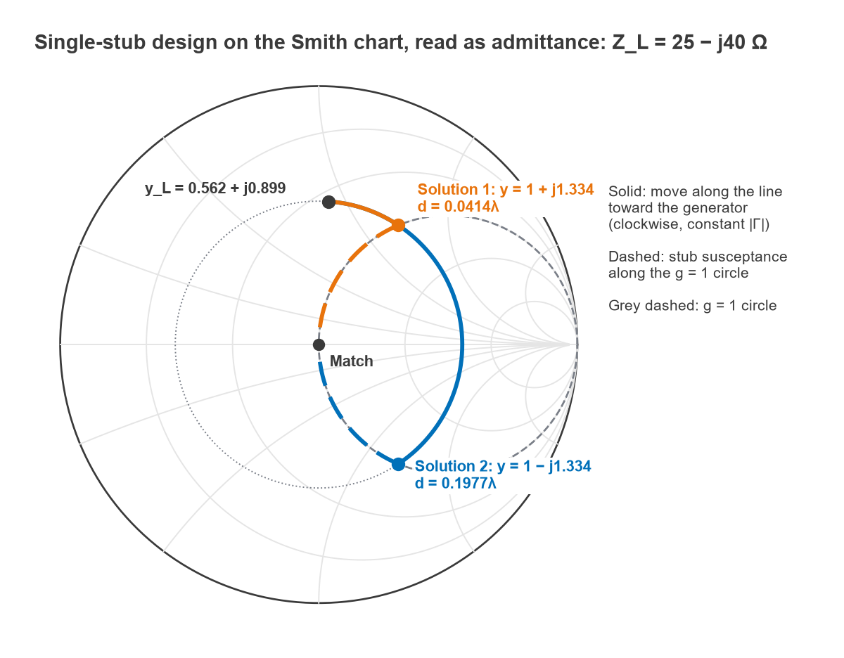
- Solution 1: t = 0.266, so d = 0.0414λ. There, y = 1 + j1.334 (B = +0.0267 S). The stub must supply −j1.334: a shorted stub of 0.1024λ, or an open stub of 0.3524λ.
- Solution 2: t = 2.934, so d = 0.1977λ. There, y = 1 − j1.334. The stub must supply +j1.334: an open stub of 0.1476λ, or a shorted stub of 0.3976λ.
Figure 1 traces both solutions. On a substrate with εr = 3.5 and h = 0.508 mm, the 50 Ω line is about 1.15 mm wide with εeff ≈ 2.75, so the guided wavelength at 2.4 GHz is 299.79/(2.4 × √2.748) = 75.4 mm. Solution 1 with a shorted stub places the stub 3.12 mm from the load, with a stub 7.72 mm long ending in a via. Solution 2 with an open stub places it 14.90 mm from the load, with a stub 11.12 mm long. Both values were checked by computing the input reflection from the exact line equations, which is zero at 2.4 GHz in every case.
Which solution to use
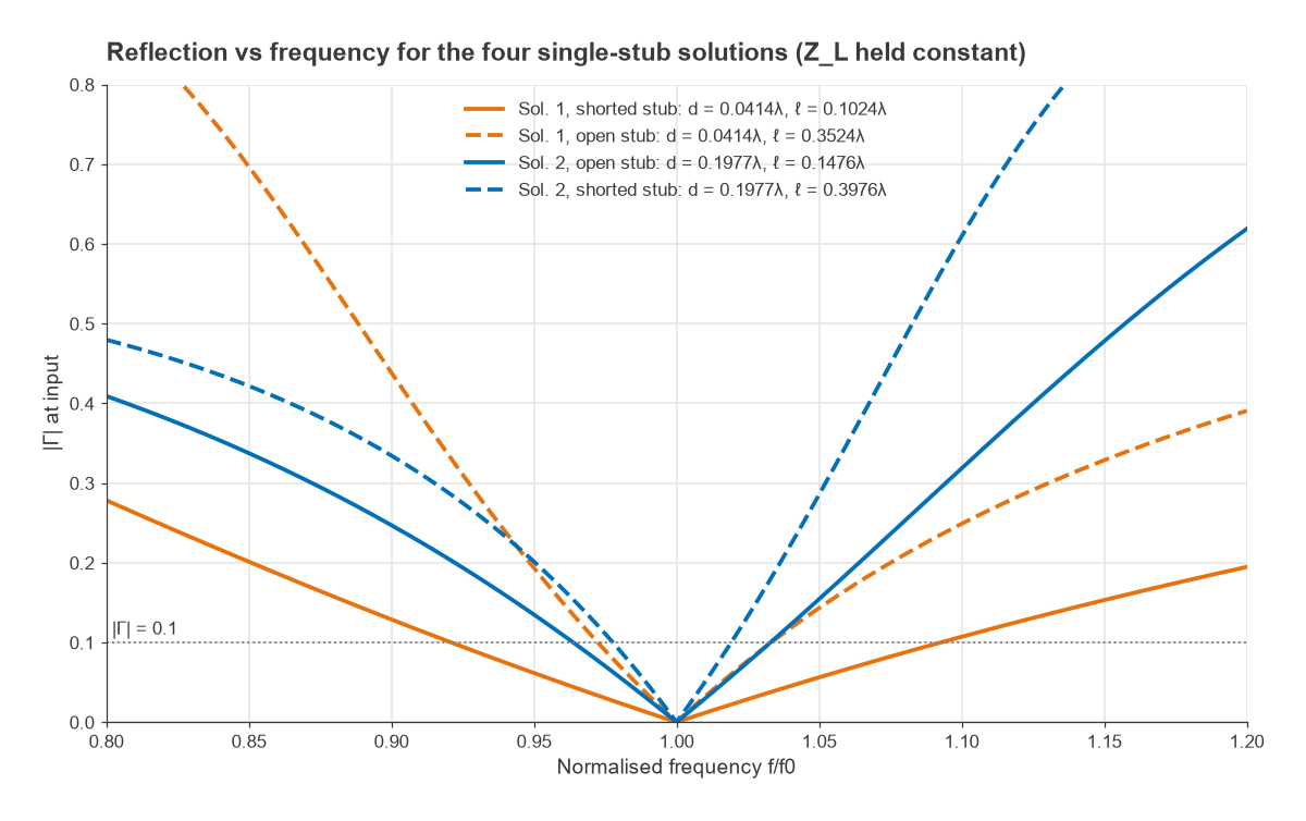
The four combinations of position and stub type all match at the design frequency, but their bandwidths differ. Figure 2 sweeps them, holding the load impedance constant so that only the matching network’s frequency dependence shows. For |Γ| ≤ 0.1 the bandwidths are 17.2% for solution 1 with a shorted stub, 6.1% for solution 1 with an open stub, 6.9% for solution 2 with an open stub and 4.2% for solution 2 with a shorted stub. The rule is general: the combination with the shortest total line length (here d + ℓ = 0.144λ) has the widest bandwidth, because the electrical lengths change least with frequency. A real load also varies with frequency, which usually narrows the result further.
Open vs shorted stubs
- Shorted stubs need a reliable connection to ground. In microstrip that means a via, whose inductance adds a little effective length. In coax and waveguide a short is clean and does not radiate, so shorted stubs are standard there. A shorted stub also provides a DC path to ground, which can serve as a bias return or ESD path, or can short a bias supply if it is not intended.
- Open stubs need no via and are easy to trim, which makes them common in microstrip. The open end has fringing capacitance that makes it look electrically longer, so the printed stub is cut slightly short; the correction is typically a fraction of the substrate thickness and is best taken from an EM simulation. In coax an open end can radiate, so open stubs are less common there.
Either type can be lengthened by any multiple of λ/2 without changing its admittance at f0, but every extra half wavelength narrows the bandwidth. The transmission line terminations page explains why open and short ends behave as they do.
Double-stub matching
A single stub must be placed at a position that depends on the load, which is awkward for an adjustable tuner. A double-stub tuner fixes the stub positions and varies only their lengths. The first stub sits at the load (or a known distance from it) and the second sits a fixed distance ds toward the generator, often λ/8 or 3λ/8.
The first stub moves the load admittance along its constant-conductance circle until it lies on the g = 1 circle rotated toward the load by ds. The line section then rotates it onto the g = 1 circle itself, and the second stub cancels the remaining susceptance. With t = tan(βds) and normalised load admittance gL + jbL at the first stub:
b1 = −bL + [1 ± √((1 + t2)gL − gL2t2)]/t, b2 = [±√((1 + t2)gL − gL2t2) + gL]/(gLt)
For the same 25 − j40 Ω load with λ/8 spacing (t = 1), the square root is √(2 × 0.562 − 0.316) = 0.899. The two solutions are b1 = +1.000 with b2 = +2.600, realised as open stubs of 0.1250λ and 0.1916λ, or b1 = −0.798 with b2 = −0.600, realised as shorted stubs of 0.1428λ and 0.1640λ.
The forbidden region
The square root must be real, which requires gL ≤ (1 + t2)/t2 = 1/sin2(βds). For λ/8 spacing that limit is gL ≤ 2: loads whose conductance at the first stub exceeds 2Y0 cannot be matched. Moving the first stub a short distance from the load, or adding a third stub, removes the problem. Spacings near 0 or λ/2 shrink the forbidden region but make the stub lengths very sensitive, so λ/8 and 3λ/8 are the usual compromises.
Radial stubs
A radial stub is a fan-shaped open stub used mainly in microstrip. Its width grows with distance from the feed point, so its characteristic impedance falls along its length. The result is an open stub that presents a low impedance, close to an RF short, over a wider band than a uniform λ/4 stub, with a shorter footprint and a well-defined feed point.
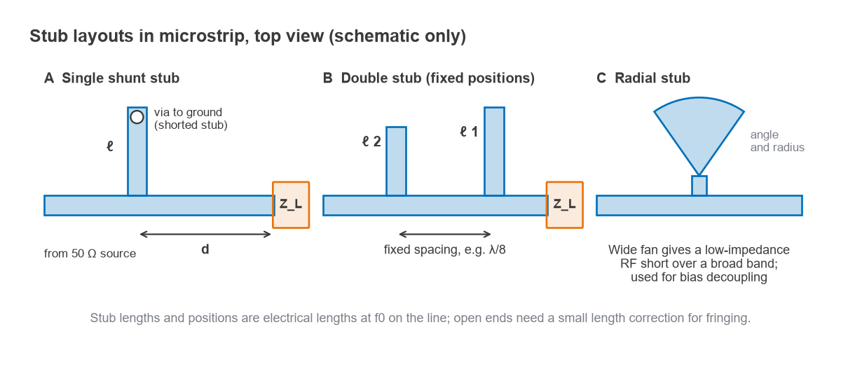
The main uses are bias networks, where a high-impedance λ/4 line feeds DC and a radial stub at its far end provides the RF short that makes the line look open at the main signal path, and broadband shunt matching elements. Design is usually by EM simulation or published closed-form models; the parameters are the radius, the fan angle (commonly in the range of about 60° to 90°) and the width of the feed line. Because the impedance varies continuously, the simple stub equations above do not apply directly. For the layout practicalities around bias feeds, see RF amplifier biasing and RF power supply decoupling.
Frequently asked questions
How do you design a single-stub match?
Convert the load to admittance, move along the line toward the generator until the conductance equals Y0, and note the distance d and the susceptance jb there. Add a shunt stub that provides −jb, using an open or shorted stub of the length that gives that susceptance.
Open vs shorted stub: which is better?
Neither is better in general. Choose the one that gives the shortest stub for the required susceptance, because shorter stubs give wider bandwidth. In microstrip, open stubs avoid vias; in coax and waveguide, shorted stubs avoid radiation from the open end.
Why can a double-stub tuner not match every load?
With fixed spacing ds, loads whose conductance at the first stub exceeds 1/sin2(βds) times Y0 cannot be brought onto the required circle. For λ/8 spacing that means conductances above 2Y0. A third stub or extra line ahead of the tuner solves it.
Related topics
The lumped equivalents are covered in L-network matching and pi and T matching networks. Line behaviour is explained in wave propagation in transmission lines, and line widths come from the microstrip calculator. For matching antennas specifically see antenna matching, and for the wider context RF design and the wireless terms glossary.