Amplifier Stability: K-Factor, Mu and Stability Circles

Amplifier stability is the property of a two-port that guarantees it will not oscillate for a given set of source and load terminations. To check it, compute the Rollett stability factor K and the determinant |Δ| from the S-parameters at every frequency where the device has gain: K > 1 with |Δ| < 1, or equivalently the single test μ > 1, means the device is unconditionally stable for any passive source and load. Anything less means some terminations will make it oscillate, and stability circles show which ones.

The tests below are part of the S-parameters branch of the RF design map, followed by a worked stabilization example checked numerically.

Why a Two-Port Oscillates

A transistor is not a one-way device. The reverse transmission S₁₂ couples some of the output back to the input through the feedback capacitance and the common-lead inductance. When that feedback combines with the source and load terminations in the right phase, the reflection coefficient looking into one of the ports exceeds unity in magnitude. A port with |Γ_in| > 1 has a negative real part of input impedance, and a negative resistance in a resonant loop is exactly what an oscillator is built from. A VCO designer wants that condition; an amplifier designer must prevent it.

For a two-port with source reflection coefficient Γ_S and load reflection coefficient Γ_L, the reflection coefficients seen at the device ports are

Γ_in = S₁₁ + S₁₂S₂₁Γ_L / (1 − S₂₂Γ_L)
Γ_out = S₂₂ + S₁₂S₂₁Γ_S / (1 − S₁₁Γ_S)

The amplifier is stable for a particular pair of terminations if |Γ_in| < 1 and |Γ_out| < 1. It is unconditionally stable if those inequalities hold for every passive source and load, that is for every |Γ_S| < 1 and |Γ_L| < 1. A device that is stable only for some terminations is called potentially unstable or conditionally stable. The S-parameters themselves, usually supplied in a Touchstone .s2p file at the intended bias, contain everything needed to decide which case applies.

The Rollett K-Factor and |Δ| Test

The classical test uses two quantities. The determinant of the scattering matrix is

Δ = S₁₁S₂₂ − S₁₂S₂₁

and the Rollett stability factor is

K = (1 − |S₁₁|² − |S₂₂|² + |Δ|²) / (2|S₁₂S₂₁|)

A two-port is unconditionally stable if and only if K > 1 and |Δ| < 1. Both conditions are needed. K > 1 on its own is not sufficient: a two-port can have K > 1 together with |Δ| > 1, and such a device is not unconditionally stable. Some texts replace the |Δ| condition with the equivalent auxiliary test B₁ = 1 + |S₁₁|² − |S₂₂|² − |Δ|² > 0.

K has a second use. When K > 1 the device can be simultaneously conjugate matched at both ports, and the resulting maximum available gain is

MAG = |S₂₁/S₁₂| (K − √(K² − 1))

When K < 1 that formula has no meaning, and datasheets plot the maximum stable gain MSG = |S₂₁/S₁₂| instead, which is the limit MAG approaches as K falls to 1. A gain curve that switches from MSG to MAG at some frequency is a direct indication of where the device crosses K = 1. The power gain definitions page treats these gain quantities in more detail.

The μ Single-Parameter Test

Edwards and Sinsky proposed a test that needs only one number. The load-plane parameter is

μ = (1 − |S₁₁|²) / (|S₂₂ − Δ S₁₁^*| + |S₁₂S₂₁|)

and the source-plane version μ′ swaps the port indices. μ > 1 (or μ′ > 1) is a necessary and sufficient condition for unconditional stability on its own. μ also has a geometric meaning: it is the distance from the centre of the Smith chart to the nearest unstable point in the load plane. That makes it useful as a figure of merit. A larger μ means the nearest unstable termination is farther away, which K does not tell you directly. Most circuit simulators provide K, B₁, μ and μ′ as built-in measurements, and it is good practice to plot all of them across the whole band where |S₂₁| > 1.

Stability Circles

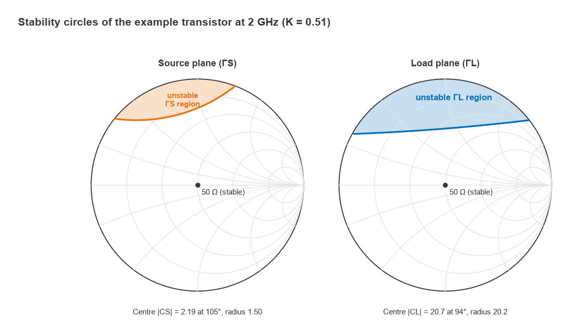
If the device is only conditionally stable, it can still be used, provided the terminations stay away from the unstable regions. The boundary |Γ_in| = 1 maps to a circle in the Γ_L plane, the output stability circle, with centre and radius

C_L = (S₂₂ − Δ S₁₁^*)^* / (|S₂₂|² − |Δ|²), R_L = |S₁₂S₂₁ / (|S₂₂|² − |Δ|²)|

Similarly, |Γ_out| = 1 maps to the input stability circle in the Γ_S plane:

C_S = (S₁₁ − Δ S₂₂^*)^* / (|S₁₁|² − |Δ|²), R_S = |S₁₂S₂₁ / (|S₁₁|² − |Δ|²)|

Deciding which side of the circle is stable takes one extra step. Consider the centre of the chart, a 50 Ω termination. With Γ_L = 0, Γ_in = S₁₁, so if |S₁₁| < 1 the centre of the load plane is stable. If the centre lies outside the output stability circle, the outside of the circle is the stable region; if the centre lies inside, the inside is stable. The same logic with S₂₂ applies to the source plane. Plotting these circles on a Smith chart alongside gain and noise circles lets a designer choose matching networks that avoid the unstable regions with some margin, because component tolerances and temperature will move both the circles and the terminations.

Worked Example: Checking a Transistor at 2 GHz

Take an illustrative small-signal transistor with these S-parameters at 2 GHz in a 50 Ω system (round numbers chosen for the example, not taken from a particular device):

S₁₁ = 0.78∠−80°, S₂₁ = 5.2∠110°, S₁₂ = 0.07∠35°, S₂₂ = 0.62∠−45°

Δ = S₁₁S₂₂ − S₁₂S₂₁ = 0.605∠−88.0°, so |Δ| = 0.605, which is less than 1.
|S₁₂S₂₁| = 0.07 × 5.2 = 0.364.
K = (1 − 0.6084 − 0.3844 + 0.3664) / (2 × 0.364) = 0.3736 / 0.728 = 0.513.
μ = 0.531 and μ′ = 0.688. Both are below 1, which agrees with K.
Output stability circle: centre 20.7∠94.5°, radius 20.2. Input stability circle: centre 2.19∠105.2°, radius 1.50.

The device is potentially unstable. |S₁₁| and |S₂₂| are both below 1, so the chart centre is stable in both planes, and since both circle centres lie farther from the origin than their radii, the stable region is outside each circle. The output circle is very large, so inside the chart it looks almost like a straight line cutting off the top of the load plane. Any load with a strongly inductive reflection coefficient in that region would drive the input into negative resistance. The maximum stable gain is 10log(5.2/0.07) = 18.7 dB, and the transducer gain in a 50 Ω system is 20log(5.2) = 14.3 dB.

Source and load plane Smith charts with shaded unstable regions for an example transistor at 2 GHz — Figure 1: Input and output stability circles of the example transistor at 2 GHz (K = 0.51). The shaded regions are terminations that cause oscillation; the chart centre is stable.

Stabilization: Resistors and Feedback

A potentially unstable device can be made unconditionally stable by adding loss or negative feedback where the device has excess gain. The four common approaches are a series resistor at the input, a shunt resistor at the output, resistive feedback from output to input, and lossy decoupling in the bias network. Each trades some gain, and sometimes noise figure or output power, for stability margin.

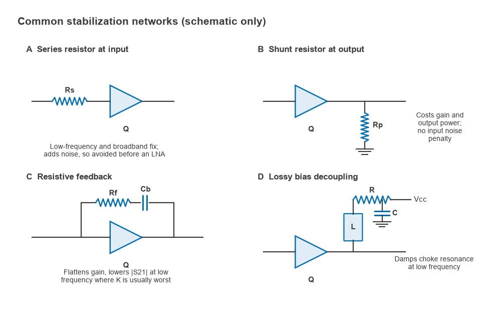
Schematic of four stabilization networks: series input R, shunt output R, RC feedback and lossy bias decoupling — Figure 3: Four common stabilization networks (schematic only).

Series resistor at the input. Very effective, especially at low frequencies, but the resistor adds its thermal noise directly at the input. It is usually avoided in the first stage of an LNA, or placed in parallel with a capacitor so it acts only below the operating band.
Shunt resistor at the output. Costs gain and some output power, but has little effect on noise figure because it sits after the gain. Often combined with a series capacitor so it loads the device only at low frequency.
Resistive feedback. An R-C network from drain to gate (or collector to base) lowers and flattens gain across a broad band. It is the standard technique in broadband amplifiers and gain blocks.
Lossy bias decoupling. A small resistor in series with the RF choke, or a resistor-capacitor pair at the cold end of the choke, damps resonances in the bias network that would otherwise present a reactive termination at low frequency.

Worked example: series input resistor

Adding a resistor R in series with the input of the example device changes its ABCD matrix by a simple cascade with [1, R; 0, 1]. Converting back to S-parameters and recomputing gives:

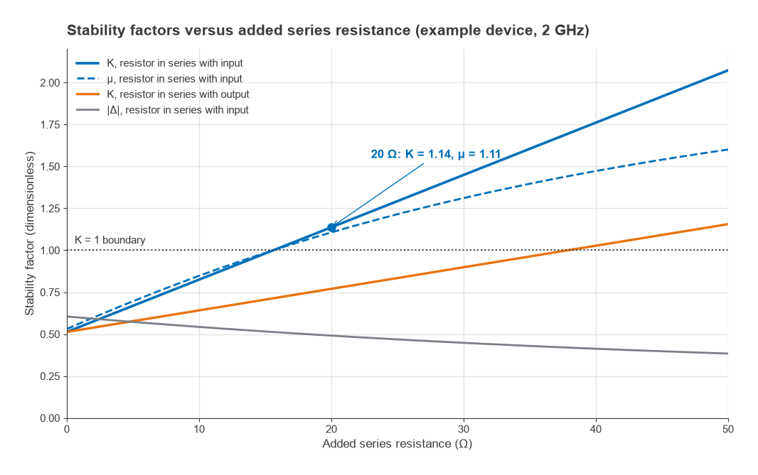
K reaches 1 at R ≈ 15.6 Ω.
With R = 20 Ω: K = 1.137, |Δ| = 0.491, μ = 1.106, μ′ = 1.099. The combination is unconditionally stable.
The 50 Ω transducer gain falls from 14.3 dB to 12.9 dB, and the maximum available gain with simultaneous conjugate match is 16.5 dB, compared with the 18.7 dB MSG of the bare device.
A resistor in series with the output is far less effective here. It needs about 38 Ω to reach K = 1, and it costs more output power.

Both stability circles move entirely outside the Smith chart once R = 20 Ω: the output circle centre becomes 4.79 with radius 3.68, and the input circle centre 3.79 with radius 2.69. A practical refinement is to bypass the resistor with a capacitor in band, keeping most of the low-frequency stability benefit while reducing the in-band gain and noise penalty.

Plot of K, mu and |Delta| versus added series resistance, with K crossing 1 near 15.6 ohms — Figure 2: K, μ and |Δ| versus added series resistance for the example device. A 20 Ω input resistor gives K = 1.14 and μ = 1.11; an output resistor needs about 38 Ω to reach K = 1.

Out-of-Band and Low-Frequency Oscillation

The most common stability failure on the bench is not at the design frequency. A bipolar or FET device often has its highest gain and lowest K well below the operating band, sometimes at tens or hundreds of megahertz, where the matching network is no longer a match and the bias chokes and decoupling capacitors form resonant circuits. A 2 GHz amplifier that tests stable at 2 GHz can oscillate at 300 MHz because the bias choke and a bypass capacitor resonate there with a high Q.

The defence is to evaluate K, μ and μ′ from the lowest frequency for which S-parameters exist up to the frequency where |S₂₁| drops below unity, using the complete circuit including bias networks, layout parasitics and via inductance. Source-lead inductance is a frequent cause of high-frequency instability in common-source FET stages, so ground vias deserve as much attention as the matching components. When an amplifier oscillates in the lab, a VNA sweep is the wrong tool; a spectrum analyzer with a wide span, looking well below and above the band, usually finds the oscillation frequency within seconds and points to the network responsible.

Multi-stage amplifiers add one more trap: stages that are each unconditionally stable can still oscillate together through shared supply lines, ground returns or coupling inside the enclosure, so the finished assembly needs checking in its housing.

Frequently asked questions

How do you check amplifier stability?

Compute K and |Δ|, or μ, from the S-parameters of the complete amplifier at every frequency where it has gain. If K > 1 and |Δ| < 1, or μ > 1, at all frequencies, it is unconditionally stable. If not, plot the stability circles and confirm the actual source and load terminations stay in the stable regions with margin.

What is K-factor?

K is the Rollett stability factor, K = (1 − |S₁₁|² − |S₂₂|² + |Δ|²) / (2|S₁₂S₂₁|). Together with |Δ| < 1, K > 1 guarantees no passive termination can cause oscillation. It also determines the maximum available gain under simultaneous conjugate match.

How do you stabilize an RF amplifier?

Add loss or feedback where the device has excess gain: a series resistor at the input, a shunt resistor at the output, R-C feedback, or resistive damping in the bias network. Making these networks frequency-selective, active mainly below the band, keeps the in-band gain and noise penalty small.