Power Gain Definitions: Transducer, Available, Operating Gain and MAG

Transducer power gain, G_T, is the ratio of the power delivered to the load to the power available from the source. It is the most complete of the two-port gain definitions because it accounts for mismatch at both the input and the output, and it is the gain an amplifier actually delivers between a real source and a real load. Operating gain, available gain and maximum available gain (MAG) are related quantities that each isolate one part of the problem.

All of these gains can be written directly from the transistor’s S-parameters and the reflection coefficients of the source and load. This page gives the formulas, shows how they relate to each other, explains maximum available and maximum stable gain, and works through a numeric example. The topic sits between S-parameter theory and RF amplifier design in the RF design reference.

Four powers and three gains

Consider a transistor described by S₁₁, S₂₁, S₁₂ and S₂₂ in a Z₀ system, driven by a source with reflection coefficient Γ_S and terminated by a load with reflection coefficient Γ_L. Any lossless matching networks are absorbed into Γ_S and Γ_L. Four power quantities can then be defined:

P_AVS, the power available from the source, delivered only into a conjugate-matched load.
P_IN, the power actually delivered to the transistor input.
P_AVN, the power available from the transistor output, which would be delivered into a conjugate-matched load.
P_L, the power actually delivered to the load.

Three gain definitions follow from them. Transducer gain is G_T = P_L/P_AVS. Operating (power) gain is G_P = P_L/P_IN. Available gain is G_A = P_AVN/P_AVS. Because P_IN can never exceed P_AVS, and P_L can never exceed P_AVN, it follows that G_T ≤ G_P and G_T ≤ G_A. G_T equals G_P when the input is conjugately matched, and equals G_A when the output is conjugately matched.

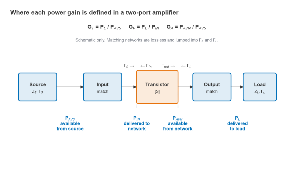
Block diagram of source, input match, transistor, output match and load with PAVS, PIN, PAVN and PL marked — Figure 1: Schematic only. The four powers that define transducer gain G_T, operating gain G_P and available gain G_A, and the reflection coefficients at the transistor ports.

The input and output reflection coefficients of the loaded transistor are needed for all three:

Γ_in = S₁₁ + S₁₂S₂₁Γ_L/(1 − S₂₂Γ_L)
Γ_out = S₂₂ + S₁₂S₂₁Γ_S/(1 − S₁₁Γ_S)

Γ_in depends on the load and Γ_out depends on the source whenever S₁₂ is not zero. That coupling through reverse transmission is what makes bilateral amplifier design harder than simply matching each port separately.

Transducer power gain G_T

Transducer gain is the quantity to use when predicting what an amplifier delivers in a system. In terms of S-parameters it is

G_T = [(1 − |Γ_S|²) / |1 − Γ_inΓ_S|²] · |S₂₁|² · [(1 − |Γ_L|²) / |1 − S₂₂Γ_L|²]

The three factors are often read as an input mismatch term, the intrinsic transistor gain and an output mismatch term. An equivalent form that uses only S-parameters and both terminations is

G_T = |S₂₁|²(1 − |Γ_S|²)(1 − |Γ_L|²) / |(1 − S₁₁Γ_S)(1 − S₂₂Γ_L) − S₁₂S₂₁Γ_SΓ_L|²

When both terminations equal Z₀, Γ_S = Γ_L = 0 and G_T reduces to |S₂₁|². That is why the S₂₁ trace on a vector network analyzer is the transducer gain of the device in a 50 Ω system, and why it is usually well below the gain the same transistor can deliver once matched.

Operating gain G_P and available gain G_A

Operating gain depends only on the load:

G_P = |S₂₁|²(1 − |Γ_L|²) / [(1 − |Γ_in|²)|1 − S₂₂Γ_L|²]

Available gain depends only on the source:

G_A = |S₂₁|²(1 − |Γ_S|²) / [|1 − S₁₁Γ_S|²(1 − |Γ_out|²)]

Each one removes a single termination from the problem, which is useful in design. Power amplifier work usually starts from the load, so constant-G_P circles on the Γ_L plane are the natural tool. Low-noise design fixes the source for minimum noise, so constant-G_A circles on the Γ_S plane are plotted alongside noise circles, as in LNA design. Once one termination is chosen, the other is set to the conjugate of the resulting Γ_in or Γ_out, and G_T then equals G_P or G_A respectively.

Maximum available gain and maximum stable gain

If the transistor is unconditionally stable, both ports can be conjugately matched at the same time: Γ_S = Γ_in* and Γ_L = Γ_out*. G_T, G_P and G_A are then equal, and their common value is the maximum available gain:

MAG = G_T,max = |S₂₁/S₁₂| · (K − √(K² − 1))

Here K is the Rollett stability factor, K = (1 − |S₁₁|² − |S₂₂|² + |Δ|²)/(2|S₁₂S₂₁|) with Δ = S₁₁S₂₂ − S₁₂S₂₁, described fully on the amplifier stability and K-factor page. MAG exists only for K ≥ 1. The required source and load reflection coefficients are

Γ_SM = [B₁ − √(B₁² − 4|C₁|²)] / (2C₁), B₁ = 1 + |S₁₁|² − |S₂₂|² − |Δ|², C₁ = S₁₁ − ΔS₂₂*

with the same form for Γ_LM after swapping the indices 1 and 2. The minus sign applies when B is positive.

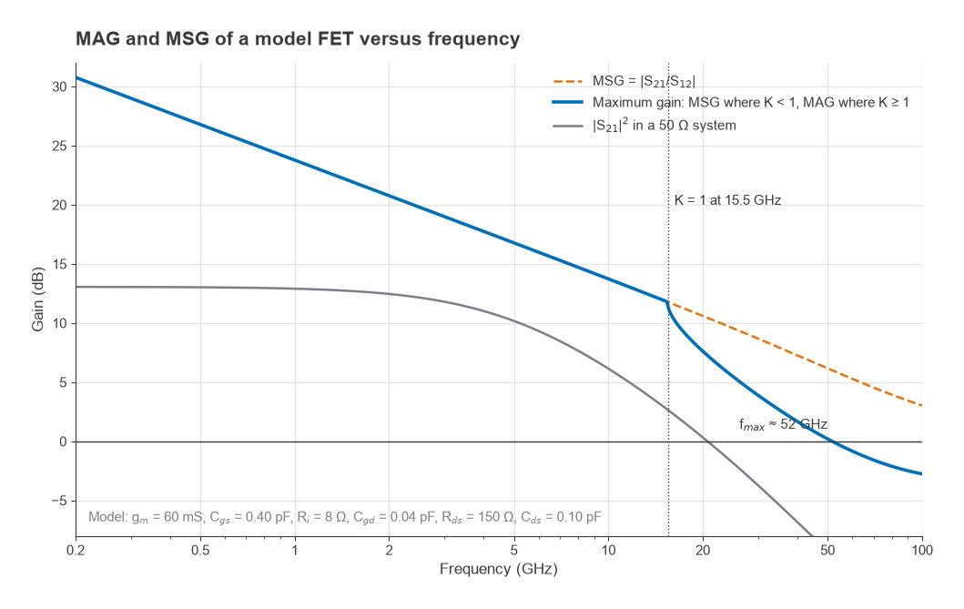
MSG, MAG and S21 squared of a model FET from 0.2 to 100 GHz, with K reaching 1 at 15.5 GHz and fmax near 52 GHz — Figure 3: Maximum gain of a simple FET model. MSG applies below 15.5 GHz where K < 1, MAG above it; the gain reaches 0 dB at f_max ≈ 52 GHz.

When K < 1 a simultaneous conjugate match does not exist, because the required terminations would make the device oscillate. The figure of merit used instead is the maximum stable gain, MSG = |S₂₁/S₁₂|. It is the value MAG approaches as K falls to 1, and it represents the gain obtainable once the device has been stabilized by just enough added loss to bring K up to 1. Datasheets often plot a single “maximum gain” curve that is MSG at low frequencies, where most transistors are potentially unstable, and MAG above the frequency where K crosses 1.

Figure 3 shows this for a simple FET equivalent circuit (g_m = 60 mS, C_gs = 0.40 pF, C_gd = 0.04 pF, R_i = 8 Ω, R_ds = 150 Ω, C_ds = 0.10 pF). MSG falls at 10 dB per decade, from 20.8 dB at 2 GHz to 13.7 dB at 10 GHz. K reaches 1 at about 15.5 GHz, where the curve switches to MAG and falls more steeply, reaching 0 dB at f_max ≈ 52 GHz. The 50 Ω |S₂₁|² is only 12.5 dB at 2 GHz, more than 8 dB below the stable gain the same device offers.

The unilateral approximation

If S₁₂ is set to zero, Γ_in = S₁₁ and Γ_out = S₂₂, and the ports can be matched independently. The unilateral transducer gain is

G_TU = [(1 − |Γ_S|²)/|1 − S₁₁Γ_S|²] · |S₂₁|² · [(1 − |Γ_L|²)/|1 − S₂₂Γ_L|²]

With Γ_S = S₁₁* and Γ_L = S₂₂* it reaches its maximum:

G_TU,max = |S₂₁|² / [(1 − |S₁₁|²)(1 − |S₂₂|²)]

Whether the approximation is acceptable is judged with the unilateral figure of merit

U = |S₁₂S₂₁S₁₁S₂₂| / [(1 − |S₁₁|²)(1 − |S₂₂|²)]

The true transducer gain then lies within 1/(1 + U)² < G_T/G_TU < 1/(1 − U)². If that error band is small, a fraction of a dB, the unilateral design is good enough and is much quicker to carry out on a Smith chart.

Worked example at 4 GHz

Take a transistor with the following S-parameters at 4 GHz in a 50 Ω system: S₁₁ = 0.72∠−116°, S₂₁ = 2.60∠76°, S₁₂ = 0.03∠57°, S₂₂ = 0.73∠−54°.

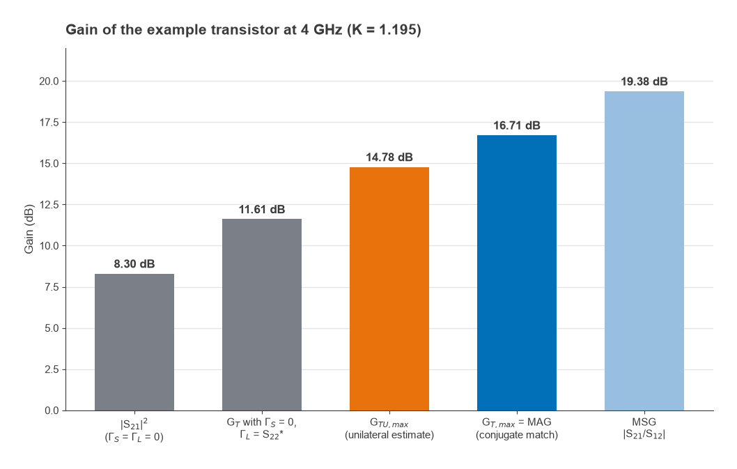
Bar chart: S21 squared 8.30 dB, partial match 11.61 dB, unilateral 14.78 dB, MAG 16.71 dB, MSG 19.38 dB — Figure 2: Gains of the 4 GHz example transistor (K = 1.195). Conjugate matching both ports lifts the gain from 8.30 dB in 50 Ω to the 16.71 dB MAG.

Stability: Δ = 0.488∠−162.3° and K = 1.195. Both K > 1 and |Δ| < 1, so the device is unconditionally stable and MAG exists.
Unmatched gain: |S₂₁|² = 6.76, or 8.30 dB.
MSG = 2.60/0.03 = 86.7, or 19.38 dB. MAG = 86.7 × (1.195 − √(1.195² − 1)) = 16.71 dB.
Simultaneous conjugate match: Γ_SM = 0.872∠123.4° and Γ_LM = 0.876∠61.0°. Substituting these into the G_T formula returns 16.71 dB, confirming MAG.
Unilateral estimate: the input term 1/(1 − 0.72²) adds 3.17 dB and the output term 1/(1 − 0.73²) adds 3.31 dB, so G_TU,max = 14.78 dB. U = 0.182, giving an error band of −1.45 dB to +1.75 dB. With Γ_S = S₁₁* and Γ_L = S₂₂* the exact G_T is 15.56 dB, inside that band but almost 1.2 dB short of MAG.

A partial design shows how the three gains differ. Leave the source at 50 Ω (Γ_S = 0) and set Γ_L = S₂₂*. The operating gain is G_P = 15.91 dB, but the loaded input reflection is |Γ_in| = 0.793, a mismatch loss of 10log(1 − 0.793²) = −4.30 dB. G_T is therefore 15.91 − 4.30 = 11.61 dB. Because the source is Z₀, Γ_out = S₂₂, the load is its conjugate, and G_A is also 11.61 dB. Figure 2 summarizes the results.

Which gain to quote

For system budgets, use G_T in the actual source and load environment, since that is what enters a cascade calculation. For comparing transistors or judging how much gain is left at a frequency, use MAG or MSG. For design, pick G_P or G_A according to which termination is constrained by another goal such as output power or noise figure. Values in dB follow the conventions described in dB and dBm explained, and the matching networks that realize Γ_S and Γ_L are covered in impedance matching and L-network matching.

Frequently asked questions

What is transducer gain?

Transducer gain is the power delivered to the load divided by the power available from the source. It includes the effect of mismatch at both ports, so it is the gain an amplifier delivers in its real environment. In a matched Z₀ system it equals |S₂₁|².

What is maximum available gain?

Maximum available gain is the transducer gain obtained when both ports of an unconditionally stable transistor are conjugately matched at the same time. It equals |S₂₁/S₁₂|(K − √(K² − 1)) and is defined only for K ≥ 1. It is the upper limit for a single stage built with lossless matching networks.

What is the difference between MAG and MSG?

MAG applies when K ≥ 1 and is achieved with a simultaneous conjugate match. MSG, |S₂₁/S₁₂|, applies when K < 1 and is the gain available after the device has been stabilized to the K = 1 boundary. At K = 1 the two values are equal.

Why is S21 lower than the gain on a transistor datasheet?

|S₂₁|² is the gain with 50 Ω on both ports, where a transistor is usually badly mismatched. Datasheet maximum gain curves show MAG or MSG, which assume ideal matching networks. In the 4 GHz example the difference is 8.4 dB.