

A gain block amplifier is a cascadable, internally matched RF amplifier, usually a 50-ohm MMIC with resistive feedback, that provides moderate, flat gain over a wide frequency range with almost no external design work. Choosing a broadband RF amplifier or gain block comes down to frequency range, gain flatness, output power (P1dB and OIP3), noise figure, port match and the supply it needs, followed by the choice between a connectorized module and a PCB-mounted part.
Unlike an LNA, which is optimised for noise, or a power amplifier, which is optimised for output power and efficiency, a broadband amplifier is optimised for consistency: the same gain and the same match across one or more octaves. That makes it the default choice for IF strips, LO chains, instrumentation and bench work. This guide sits in the RF amplifiers section; the circuit techniques behind these parts are covered in Broadband RF Amplifier Design.
What Makes an Amplifier a Gain Block
Most gain blocks use a Darlington pair or a single transistor with shunt and series resistive feedback. The feedback trades some of the transistor’s available gain for input and output impedances close to 50 ohms over a wide band and for gain that is nearly independent of frequency until the device itself runs out of bandwidth. The result can be cascaded with DC blocking capacitors and a bias feed, and nothing else. The price of the feedback resistors is a noise figure of a few dB rather than a fraction of a dB, and DC power that is often higher than an LNA’s for the same gain.
Broadband amplifier is the wider term. It also covers balanced amplifiers, distributed amplifiers and connectorized modules that may contain several gain stages. The selection criteria below apply to all of them.
Specifications That Matter
The ranges in the table are approximate and reflect common datasheet values for general-purpose parts, not limits.
| Specification | Why it matters | What to look for |
|---|---|---|
| Frequency range | Gain and match are only guaranteed inside it | Covers the band with margin at both ends; check where the low-frequency limit comes from (device or coupling capacitors) |
| Gain and gain flatness | Sets level and amplitude accuracy across the band | Gain commonly 10 to 25 dB per stage; flatness quoted over a stated sub-band, often well under ±1 dB |
| Noise figure | Matters if the amplifier is early in a receive chain | Commonly around 2 to 6 dB for feedback gain blocks |
| P1dB | Maximum usable output before compression | Well above the highest output level the application needs |
| OIP3 | Intermodulation with multiple signals | Roughly 10 dB or more above P1dB for many feedback designs |
| VSWR / return loss | Mismatch loss and ripple with cables and loads | Return loss of 10 dB or better (VSWR below 2:1) at both ports |
| Reverse isolation | Leakage back toward the source | Often comparable to the forward gain in feedback designs; check it for LO and isolation uses |
| Supply | Bias network, power budget and heat | Supply voltage, current, whether a bias resistor and choke are needed |
Reading gain flatness correctly
Figure 1 models a feedback gain block with 20 dB of mid-band gain, a low-frequency corner at 10 MHz set by coupling capacitors and a high-frequency corner at 4 GHz set by the device. Between 50 MHz and 1 GHz the gain varies by only 0.24 dB. Stretch the band to 2 GHz and the variation grows to 0.94 dB, because the response is already rolling off at the upper end. A flatness figure is only meaningful together with the band it applies to, and a part that is perfectly flat in the middle of its range may be several dB down at the frequency you care about. When gain at the band edge matters, read the gain-versus-frequency plot, not the summary table.
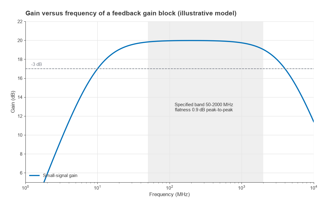
The low-frequency corner of a PCB-mounted gain block is often set by the coupling capacitors and the bias choke, not by the device. Larger capacitors and a choke with higher inductance extend the response downward, and a poor choke with a self-resonance inside the band produces a notch or a gain spike.
Port Match and Mismatch Ripple
A broadband amplifier rarely drives a perfect load. The reflection coefficient at each port is Γ = (VSWR − 1)/(VSWR + 1), and when an amplifier output with reflection Γ1 drives a load with reflection Γ2, the delivered power can vary between the limits
ΔG = 20log(1 ± |Γ1||Γ2|)
depending on the phase of the reflections, which changes with frequency and cable length. Over a wide band that phase sweeps through every value, so the limits appear as ripple on a gain plot.
Worked example: ripple from a 2:1 match
- VSWR 2:1 gives |Γ| = 1/3, a return loss of 9.54 dB and a mismatch loss of 0.51 dB on its own.
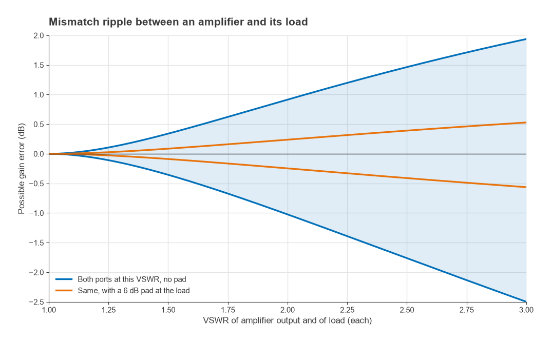
- If both the amplifier output and its load are 2:1, |Γ1||Γ2| = 0.111, and the ripple limits are +0.92 dB and −1.02 dB, a span of almost 2 dB.
- A 6 dB attenuator at the load improves its apparent return loss by 12 dB (the reflection passes through the pad twice), to 21.5 dB. The ripple limits shrink to +0.24 dB and −0.25 dB.
- At VSWR 1.5:1 on both sides, without a pad, the limits are +0.34 dB and −0.35 dB.
The mismatch ripple from two 2:1 ports is already larger than the 0.94 dB flatness of the amplifier itself. In bench work this is the usual reason a measured frequency response looks worse than the datasheet. Pads at the amplifier ports are the simplest fix, at the cost of output level. The theory is covered in VSWR and Return Loss.
Output Power, Harmonics and Linearity
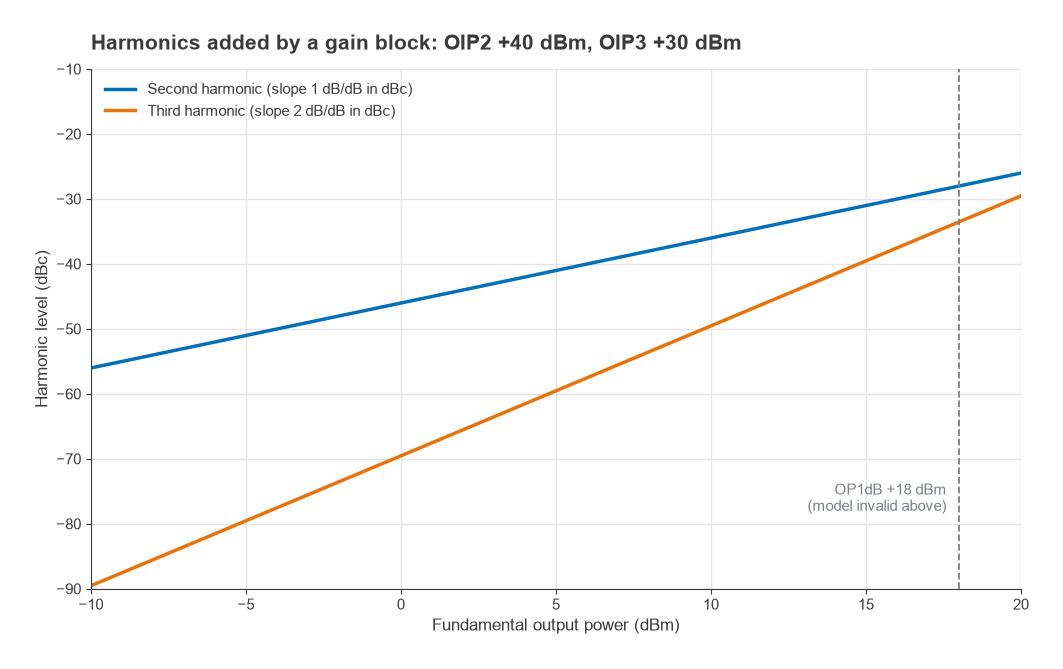
A broadband amplifier passes its own harmonics as readily as the fundamental. If the amplifier covers 50 MHz to 2 GHz and the signal is at 300 MHz, the second and third harmonics at 600 and 900 MHz are amplified with full gain. Their levels follow from the intercept points. For an output tone Pout, referred to the carrier:
- Second harmonic: H2 ≈ Pout − OIP2 − 6 dBc
- Third harmonic: H3 ≈ 2Pout − 2·OIP3 − 9.5 dBc
The 6 dB and 9.5 dB offsets come from the power-series model: a single-tone harmonic is half the amplitude of the corresponding two-tone second-order product, and one third of the corresponding third-order product. For a gain block with OIP2 = +40 dBm and OIP3 = +30 dBm, an output of +10 dBm gives H2 ≈ −36 dBc and H3 ≈ −49.5 dBc. At 0 dBm they improve to −46 dBc and −69.5 dBc. For anything that needs a clean signal, either run well below P1dB or add a low-pass filter after the amplifier. The P1dB and harmonic distortion pages explain the underlying model.
Connectorized Module or PCB MMIC?
| Factor | Connectorized module | PCB-mounted MMIC |
|---|---|---|
| Integration effort | None; cable in, cable out, apply DC | Layout, bias network, coupling capacitors, grounding |
| Performance control | Fixed by the module design | Depends on board material, layout and bias choke |
| Size and cost per channel | Larger, higher | Small, low |
| Protection | Often includes regulation, reverse-polarity protection and shielding | Whatever the designer adds |
| Typical use | Bench setups, test systems, prototypes, one-off links | Products, multi-channel designs, anything built in volume |
For a test bench, a connectorized module saves days of layout and measurement. For a product, the same MMIC on a well-designed board performs as well at a fraction of the size, provided the ground vias, the bias choke and the transmission lines are done properly. Guidance on those details is in Biasing RF Transistors and MMICs and in the RF PCB layout guides.
Test Bench Uses
Driving a mixer LO port
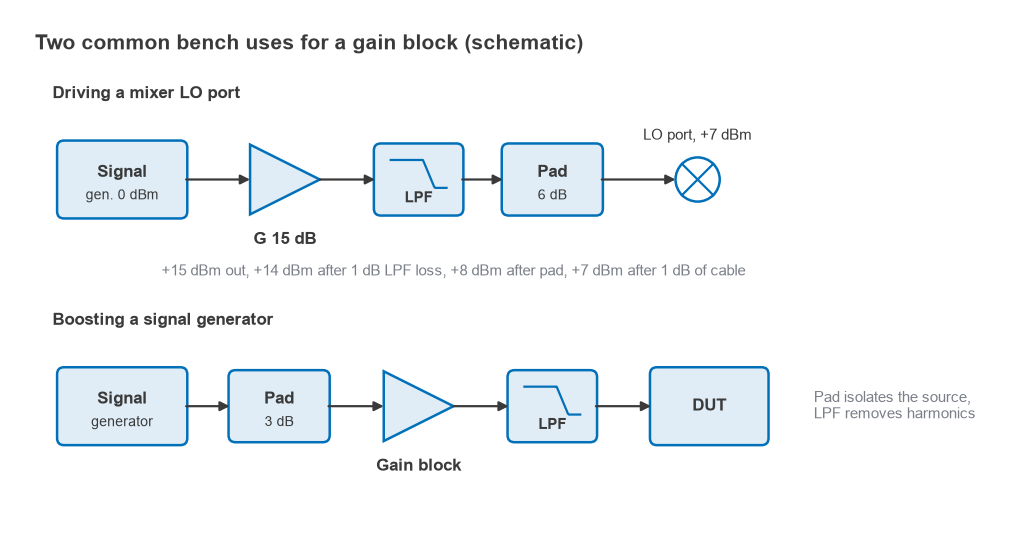
Passive diode mixers commonly need an LO drive of around +7 dBm or more, while many signal generators and synthesiser boards deliver less. Suppose the source gives 0 dBm. A gain block with 15 dB gain and OP1dB = +18 dBm raises it to +15 dBm, 3 dB below compression. A low-pass filter with 1 dB loss removes the harmonics (at +15 dBm, the model above puts H2 at about −31 dBc), a 6 dB pad brings the level to +8 dBm and presents the mixer with a better-matched source, and 1 dB of cable delivers +7 dBm. LO drive tolerates some compression, but harmonics on the LO change the mixer’s spur behaviour, so the filter is worth keeping.
Boosting a signal generator
When a generator cannot reach the level a test needs, a gain block after it is the obvious solution. Three precautions keep the result trustworthy. Put a small pad between the generator and the amplifier so the generator’s level control sees a stable load. Keep the amplifier well below P1dB, because the generator’s level accuracy and modulation quality are lost in compression. Add a low-pass filter after the amplifier when harmonic content matters, since the amplifier’s harmonics may exceed the generator’s own specification. Measure the actual level at the device under test with a power meter, as described in Measuring Amplitude and Power in RF Signals.
Selection Checklist
- The specified frequency range covers the band, and the gain plot shows acceptable gain at both band edges.
- Gain flatness is specified over the sub-band you will use.
- P1dB exceeds the highest required output level by several dB; OIP3 suits the number and level of signals present.
- Noise figure is acceptable if the amplifier sits early in a receive chain.
- Port VSWR, combined with the source and load match, gives tolerable ripple; pads are planned where it does not.
- Supply voltage and current fit the available power, and the bias network suits the lowest operating frequency.
- Connectorized or PCB form suits the project stage and volume.
- A harmonic filter follows the amplifier wherever spectral purity matters.
Frequently asked questions
What is a gain block amplifier?
A gain block is a broadband amplifier that is internally matched to 50 ohms, usually through resistive feedback, so it can be cascaded with only coupling capacitors and a bias feed. It offers flat, moderate gain over a wide band at the cost of a higher noise figure than a dedicated LNA.
What specs matter for a broadband amplifier?
Frequency range, gain and gain flatness over the band in use, P1dB and OIP3, noise figure if it is in a receive path, input and output VSWR, and supply requirements. Port match deserves more attention than it usually gets, because mismatch ripple can exceed the amplifier’s own flatness.
Should I use a connectorized amplifier or a PCB MMIC gain block?
Use a connectorized module for bench work, test systems and prototypes, where integration time matters more than size or unit cost. Use a PCB-mounted MMIC for products and multi-channel designs, accepting that layout, grounding and the bias network then become your responsibility.
Can a gain block replace an LNA?
Where the antenna noise is high, as at HF and in many VHF systems, a gain block’s few dB of noise figure makes little difference to sensitivity. For satellite, GNSS and other low-noise applications, a dedicated LNA gives a clear improvement.
Related topics
Compare the three main amplifier roles in LNA vs Gain Block vs Power Amplifier, learn to interpret test conditions in How to Read an RF Amplifier Datasheet, and see how stages combine in cascaded IP3. The full reference starts at RF design.