

Harmonic balance is a frequency-domain circuit simulation method that finds the periodic steady state of a nonlinear circuit directly, by representing every node voltage as a sum of harmonics and solving for their amplitudes until the currents in the linear and nonlinear parts of the circuit balance at each frequency. Unlike transient simulation, it does not step through the start-up, so it handles high-Q networks, distributed elements and closely spaced tones efficiently.
Harmonic balance is one of four simulation methods an RF designer uses routinely, alongside S-parameter (small-signal AC) analysis, circuit envelope and transient. Each answers a different question, and using the wrong one costs either accuracy or hours of run time. This page belongs to the RF engineering tools section of the RF design guide. It explains how harmonic balance works, compares the methods, and quantifies why transient simulation struggles with typical RF problems.
How Harmonic Balance Works
Assume the circuit is driven by one periodic source at f0 and has reached steady state. Every node voltage can then be written as a truncated Fourier series,
v(t) = Re{ Σk=0…K Vk ejkω0t }
where K is the number of harmonics kept. The circuit is split into a linear part and a nonlinear part. The linear part, which can include lumped elements, transmission lines, measured S-parameter blocks and EM-simulated layouts, is described exactly in the frequency domain by its admittance matrix at each harmonic. The nonlinear devices, such as transistor and diode models, are described by current and charge equations in the time domain.
Each iteration converts the current estimate of the harmonic voltages to a time waveform with an inverse FFT, evaluates the nonlinear currents i(t) and charges q(t), and transforms those back to the frequency domain. Kirchhoff’s current law must then hold at every node and every harmonic:
F(V) = Y·V + INL(V) + jΩ·QNL(V) − IS = 0
Here Y is the linear admittance matrix, Ω is a diagonal matrix of the harmonic frequencies kω0, and IS holds the source currents. A Newton-Raphson solver drives the error F(V) toward zero. The unknown vector has roughly N × (2K + 1) real entries for N nodes, so the Jacobian grows quickly with harmonics. Modern simulators use Krylov iterative solvers to handle large circuits without forming the full matrix.
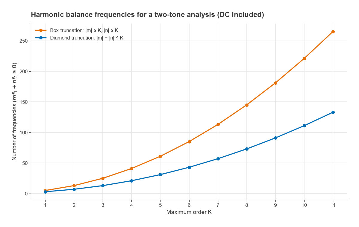
The method extends to several incommensurate tones, for example two closely spaced input tones, an RF and an LO, or a signal and a blocker. The frequency set then becomes every mix m·f1 + n·f2 within a chosen truncation. A diamond truncation keeps |m| + |n| ≤ K and is usually enough for intermodulation work; a box truncation keeps |m| ≤ K and |n| ≤ K and is used in mixers where high LO harmonics matter.
The Four Main RF Simulation Methods
S-parameter and AC analysis
The circuit is linearized around its DC bias point and solved at each frequency. This is fast and exact for linear behaviour: gain, match, stability, noise figure and group delay. It is the right tool for filters, matching networks, couplers and small-signal amplifier design, and its outputs connect directly to S-parameters and stability analysis. It says nothing about compression, harmonics or intermodulation.
Harmonic balance
The method for steady-state nonlinear behaviour with periodic or few-tone excitation. Typical uses are output power and efficiency of a power amplifier, the 1 dB compression point, IP3 from two-tone tests, simulated load-pull contours, mixer conversion gain and spurs, and oscillator frequency, output power and phase noise. Large-signal noise analysis around the HB solution is how simulators predict mixer noise figure and phase noise.
Circuit envelope
Envelope analysis is harmonic balance with time-varying harmonic amplitudes. Each harmonic carries a complex envelope Vk(t), and the simulator steps in time at a rate set by the modulation bandwidth, not the carrier. For a modulated signal of bandwidth B, the envelope time step is on the order of 1/(several × B). A 20 MHz wide signal on a 3.5 GHz carrier therefore needs steps of a few nanoseconds rather than picoseconds. It is used for ACLR, EVM, memory effects, AGC and PLL loop transients, and turn-on behaviour of pulsed amplifiers.
Transient
Transient analysis integrates the circuit equations step by step in time, as SPICE does. It makes no assumption about periodicity, so it handles start-up, strongly switching circuits, digital logic, charge pumps, sampling circuits and arbitrary waveforms. Its weaknesses for RF are run time with high-Q or slowly settling circuits, and difficulty with frequency-domain models such as dispersive transmission lines and measured S-parameter files, which must be converted to time-domain impulse responses that may not be causal or passive.
Comparison Table
| Method | Domain | Signal type | Typical outputs | Main limitation |
|---|---|---|---|---|
| S-parameter / AC | Frequency | Small signal | Gain, match, NF, stability | Linear only |
| Harmonic balance | Frequency | Periodic, a few tones | Pout, PAE, P1dB, IP3, spurs, phase noise | Strong switching needs many harmonics |
| Circuit envelope | Mixed | Modulated carriers | ACLR, EVM, transient envelope | Longer run time than HB |
| Transient | Time | Arbitrary | Start-up, switching, digital | Slow for high Q, poor with S-parameter data |
Worked Example: Why Transient Struggles at RF
Consider a 1 GHz amplifier with an output network of loaded Q = 50. The amplitude envelope of a resonant circuit settles with time constant τ = 2Q/ω0.
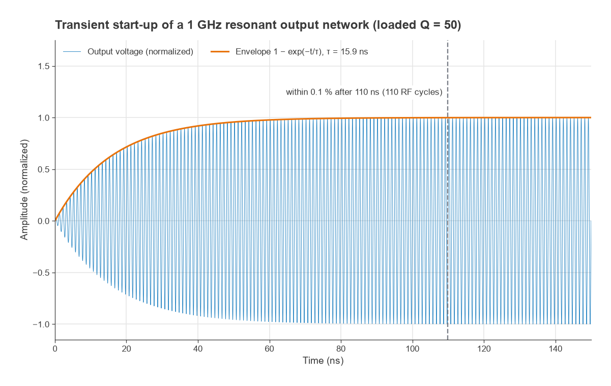
- τ = 2 × 50 / (2π × 109) = 15.9 ns.
- Settling to within 0.1 % (60 dB) takes ln(1000) × τ = 6.91 × 15.9 = 110 ns, or 110 RF cycles.
- To resolve the fifth harmonic with 20 points per period, the time step is 1/(5 × 109 × 20) = 10 ps, so about 11,000 steps are needed before the first useful cycle.
That is manageable for a single tone. Now add a second tone 1 MHz away to measure intermodulation. The combined waveform repeats only every 1/Δf = 1 µs, so transient needs at least 1 µs of settled data, which at 10 ps per step is 100,000 steps on top of the settling time, followed by an FFT with careful windowing to see products 60 dB or more below the tones. Harmonic balance solves the same problem directly on a small frequency set. With diamond truncation at K = 7, the two-tone analysis uses 57 frequencies, including DC.
What the two-tone HB result looks like
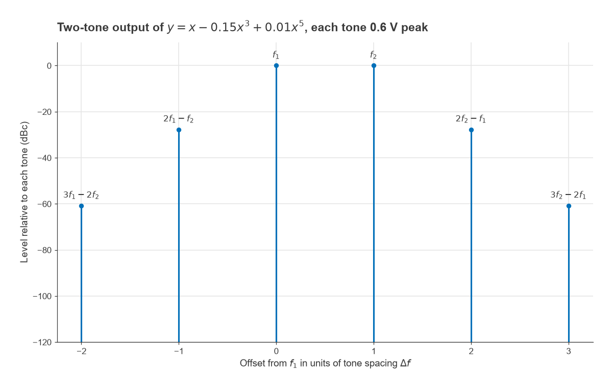
For a memoryless nonlinearity y = x − 0.15x3 + 0.01x5 driven by two equal tones of 0.6 V peak, the output tone amplitude is a1A + (9/4)a3A3 + (25/4)a5A5 = 0.600 − 0.0729 + 0.0049 = 0.532 V. The third-order product is (3/4)a3A3 + (25/8)a5A5 = −0.0243 + 0.0024 = −0.0219 V, which is 27.7 dB below each tone. The fifth-order products at 3f1 − 2f2 and 3f2 − 2f1 come out 60.8 dB down. An FFT of the exact time waveform gives the same values, which is a useful sanity check on any simulator setup.
When to Use Each Method
- Small-signal design and passive networks: S-parameter analysis, with EM-simulated layout where needed. See EM simulation basics.
- Power, compression, harmonics, IMD, mixers and oscillators in steady state: harmonic balance.
- Realistic modulated signals and slow control loops: circuit envelope, often seeded with an HB solution.
- Start-up, switching converters, digital interfaces, pulse shapes and anything non-periodic: transient.
Harmonic balance becomes harder when the circuit switches hard. A class E or class D stage, a hard-limited mixer or a frequency divider produces waveforms with sharp edges and needs many harmonics, which slows HB and can stop it converging. Those circuits are often run first in transient to understand the waveforms, then in HB with a high harmonic count once the design is close. Oscillators need special handling in HB because the frequency is an unknown; simulators add it to the solution vector and usually need an initial guess near the expected frequency. The VCO design page covers oscillator conditions in more detail.
Convergence tips
- Ramp the input power in steps (source stepping) rather than starting at full drive.
- Increase the harmonic order until output power and the products of interest stop changing by more than a small fraction of a decibel.
- Check that the oversampling of the FFT is sufficient for strongly nonlinear device models.
- Keep a DC and S-parameter check of the same schematic. If those are wrong, HB will be wrong too.
Frequently Asked Questions
What is harmonic balance?
Harmonic balance is a nonlinear simulation method that solves for the steady-state amplitudes of a set of harmonics and mixing products directly in the frequency domain. It balances linear-network currents, calculated in the frequency domain, against nonlinear-device currents, calculated in the time domain, using Newton iteration.
Is harmonic balance faster than transient?
For steady-state RF problems with high-Q networks, distributed elements or closely spaced tones it is usually much faster, because it skips the start-up and the long beat period. For strongly switching circuits that need hundreds of harmonics, transient can be competitive or better.
Can SPICE do harmonic balance?
Classic SPICE is a transient and AC simulator. Some open-source and commercial simulators add harmonic balance or periodic steady-state analysis, which is the time-domain counterpart based on shooting methods. The free RF design software and RF simulation software pages compare what is available.
How many harmonics should I use?
Enough that the results stop changing. Mildly nonlinear amplifiers often converge with 5 to 9 harmonics, while saturated PAs, mixers and dividers may need many more. A two-tone run with diamond truncation at order 7 uses 57 frequencies.
Related Topics
The tools and resources hub links the other software pages, including Python for RF engineers with scikit-rf and the RF calculators. For the nonlinear quantities HB predicts, see RF linearity, harmonic distortion and AM-PM and mixer types.